Documentation
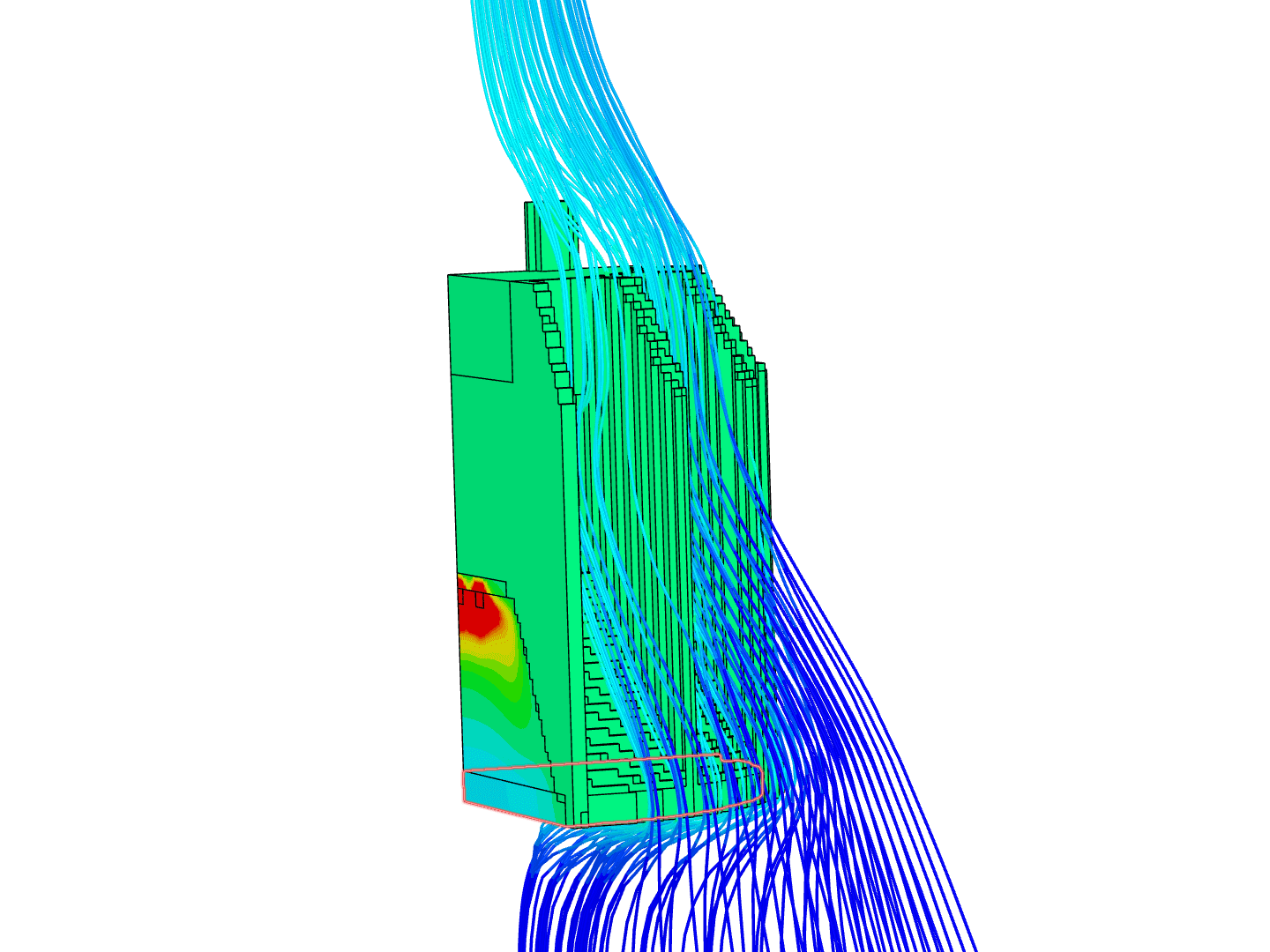
The Conjugate Heat Transfer (IBM) (Immersed Boundary Method) analysis type allows for the simulation of heat transfer between solid and fluid domains by exchanging thermal energy at the interfaces between them. Typical applications of this analysis type exist as but are not limited to, the simulation of heat exchangers, cooling of electronic equipment, and general-purpose cooling and heating systems.
The difference to the Conjugate Heat Transfer is that the IBM is resilient to complex geometrical details and does not require CAD simplification.
The following section will explain the step-by-step procedure to set up a conjugate heat transfer (IBM) simulation within the SimScale platform:
To create a CHT (IBM) analysis, first, select the desired geometry and click on ‘Create Simulation’:
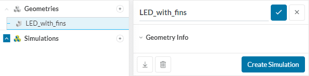
Please note that .stl models are not supported for CHT (IBM) analyses. A list of alternative supported CAD formats can be found here.
Next, a window with a list of analysis types supported in SimScale will be displayed:
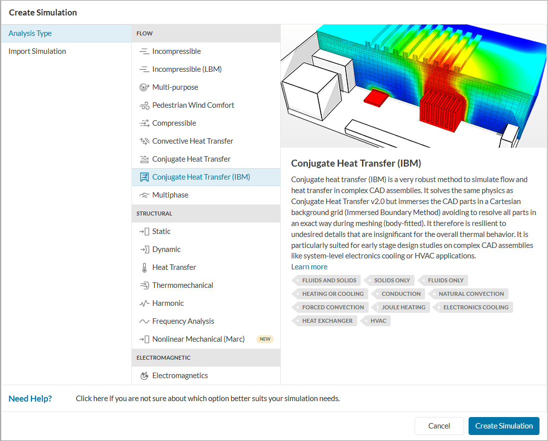
Choose Conjugate Heat Transfer (IBM) analysis type and click on ‘Create Simulation’. This will lead to Workbench for the simulation with the following simulation tree and the respective settings:
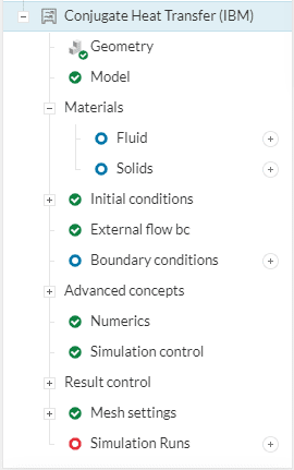
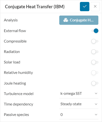
To access the global settings, click on ‘Conjugate Heat Transfer (IBM)’ in the simulation tree. It consists of certain parameters that can be selected to define the simulation. The parameters are listed below:
Find detailed information on each parameter here.
When performing a Conjugate Heat Transfer (IBM) analysis, no additional CAD requirements have to be taken into account. In addition, the creation of an external flow domain is not necessary when the External Flow option is activated under Global Settings. Otherwise, please create the internal or external flow domain within the CAD Edit environment.
This knowledge-based article explains how to create the internal or external flow domain within the CAD Edit environment.
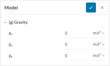
Under Model, the gravitational direction and magnitude can be defined. When performing a thermal analysis it’s recommended to consider gravity as buoyancy has an influence on the temperature distribution within a fluid.
The CHT (IBM) analysis type allows you flexibility with the materials being used in the simulation. It can be used with only flow regions, only solids, or a combination of both.
Users can now run conjugate, convective, and simple heat transfer simulations within CHT (IBM), to leverage its handling of non-simplified geometry for other types of simulations. Read more in the dedicated document on materials in SimScale.
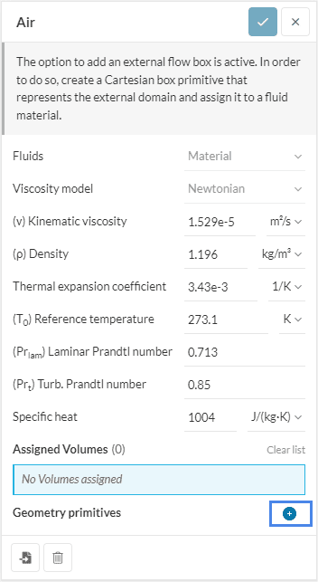
When External Flow is activated under Global Settings an external flow domain needs to be defined. However, no CAD geometry is necessary, as it can be defined via a geometry primitive, which is then assigned to the fluid material. To create a new geometry primitive click on the plus icon at the bottom of the settings panel of the fluid material properties.
In a conjugate heat transfer simulation, the computational domain will be solved for three fields: pressure \((P)\) and velocity \((U)\), and temperature \((T)\). Here the pressure is referred to as Modified gauge pressure or Modified pressure when compressible fluid is activated. While Modified Gauge Pressure is given relative to the ambient pressure Modified pressure is given as absolute pressure. Additional turbulent transport quantities may be included based on the turbulence model selected. Under Initial conditions, these values can be initialized for the whole domain or a sub-domain for each region.
Important
For any simulation, initial and boundary conditions must be specified for all required variables on every boundary.
It is recommended to set the initial conditions close to the expected solution to avoid potential convergence problems. Learn more about initial conditions in this document.
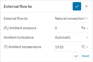
When the external Flow boundary condition is activated the boundary conditions will be applied to all faces of the flow domain. The user can choose between a natural convection inlet/outlet or a wall boundary condition. When a symmetrical boundary should be applied to the fluid volume it’s necessary to create the fluid Volume within the Edit in CAD Mode.
Boundary conditions help to add closure to the problem at hand by defining how a system interacts with the environment. Following is a list of links to the available boundary conditions documentation each explaining their importance and how they can be applied to the domain boundaries.
Some boundary conditions available in conjugate heat transfer simulations are supported in parametric experiments. Find more details about parametric studies in this article.
Important
In case no boundary conditions are assigned to a face, by default it will receive a no-slip wall boundary condition with wall function for turbulence resolution, and adiabatic thermal behavior.
Under Advanced Concepts, you will find additional setup options, the available options are:
Visit this dedicated page for more information.
Furthermore, momentum sources, power sources, and rotating zones are supported in parametric experiments. This dedicated article contains more information on parametric studies.
Numerical settings play an important role in the simulation configuration. They define how to solve the equations by applying proper discretization schemes and solvers to the equations. They help enhance the stability and robustness of the simulation. Although all numerical settings are made available for users to have full control over, it is advised to keep them default unless necessary.
Note
SimScale uses its own version of OpenFOAM® solvers developed in-house.
Numerical settings are recommended for advanced users but interested readers are encouraged to learn more about them through this documentation.
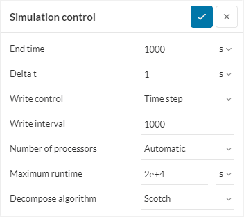
The Simulation Control settings define the general controls over the simulation. In these settings, the number of iterations, simulation interval, timestep size, and several other variables can be set. Find further information here.
The Result Control section allows users to define additional simulation result outputs. It controls how the results will be written, meaning the write frequency, location, statistics of the output data, etc. The available options are as follows:
Find more details about result controls here.
Meshing is the process of discretization of the simulation domain. That means we split up a large domain into multiple smaller domains and solve equations for them.
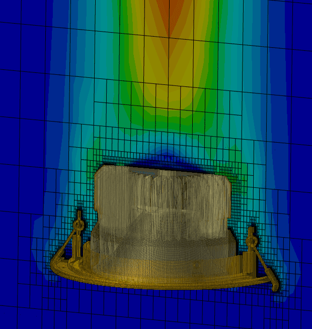
The Immersed Boundary simulations are based on Cartesian meshes. These do not resolve every part separately as in a body-fitted meshing approach but refine the cartesian grid towards geometrical and topological details and immerse the geometry into it. The detailed treatment is done on the solver level instead.
The above-discussed meshing approach has some strong advantages:
In CHT (IBM) three different methods to define the size of your mesh are available. For each meshing method, it is also possible to add a regional refinement or a local element size refinement.
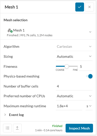
With the automatic setting, you can quickly set up mesh by choosing a level of fineness. The range goes from 0 (coarse) to 10 (fine), with a high number resulting in a finer mesh.
Automated Mesh Sensitivity Study
For the automatic meshing the fineness level of the mesh can be used in a parametric study allowing for fast automatic mesh sensistivy studies.
Manual Meshing allows you to define the maximum and minimum edge lengths of a cell.
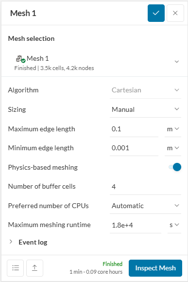
Maximum edge length
The Maximum edge length defines the biggest cell size in the mesh and therefore the unrefined level 0. The mesh will be automatically refined where geometrically or physically helpful.
Minimum edge length
The Minimum edge length defines the smallest cell size except for local refinements. As refinements are based on cell splits (1 –> 8 cells) the actual smallest size might differ slightly from the chosen value.
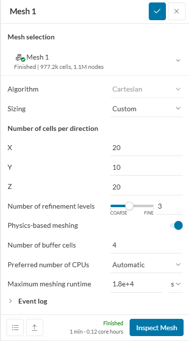
For a custom mesh, the number of cells per direction has to be defined, as well as the number of refinement levels. The number of refinement levels defines the smallest cell size, as for each level the cell size is divided in half.
Last updated: April 3rd, 2026
We appreciate and value your feedback.
Sign up for SimScale
and start simulating now