Simulation Control for Fluid Analysis
Ever wondered what those technical terms inside the Simulation control settings panel mean? If yes, then this is the right place to get all your queries answered. This document gives detailed explanations for the settings that control the simulation run in SimScale, specifically for the fluid simulation analysis types supported with the OpenFOAM® solver and the Multi-purpose analysis type as well.
Following analysis types are based on the OpenFOAM® solver:
- Incompressible
- Compressible
- Convective Heat Transfer
- Conjugate Heat Transfer
- Conjugate Heat Transfer (IBM)
- Multiphase
One should find the following control settings:
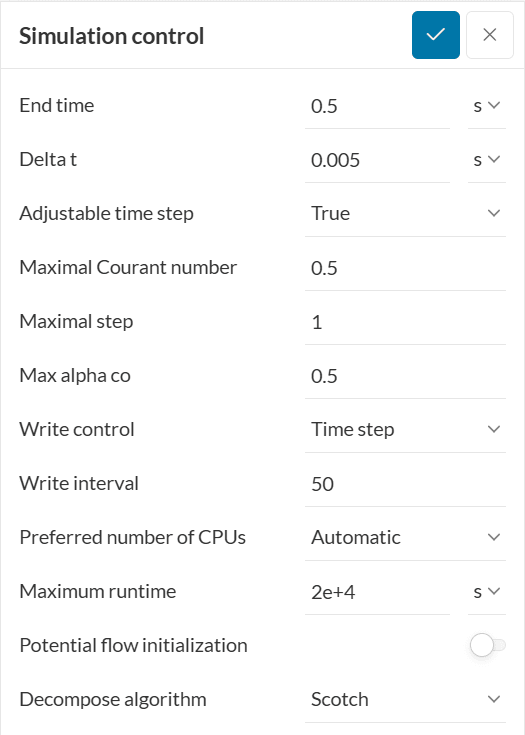
End Time
Steady State
Steady state simulations are time-independent, that is, the equations solved do not include time derivatives. Hence, End time here represents end of the simulation. No more iterations will be executed beyond this value.
Transient
Transient simulations depend on time. The associated flow variables vary with respect to time. Hence, End time represents the time for which the transient effects need to be analyzed in any physical phenomenon. For transient simulations, End time is often referred to as the simulation time.
Delta T
Steady State
For steady state simulations, Delta t represents the iteration step size. In other words, it reflects how aggressively you want to reach the end of simulation. It is also referred to as pseudo-time step. Hence,
$$Number\ of\ iterations = \frac{End\ time}{Delta\ t}$$
Note
Although there can be different combinations of End time and Delta t for the same Number of iterations it is advised to keep the step size small (usually 1).
Transient
For transient simulations, Delta t is the incremental change in time for which the transient equations are solved during the simulation run. It is commonly referred to as time step or time step size.
Steady state vs Transient
Number of iterations has a different meaning when using steady state and transient. For transient, number of iterations means sub-iterations within each timestep.
In transient simulations a given timestep is assumed to be converged if the residuals fall below a given value.
Adjustable Time Step
For transient simulations, it is possible to adjust the time step Delta t by setting the Adjustable time step option to True. This means that in spite of defining a time step value it will still be adjusted based on the maximum value of Courant number and the maximum allowed time step.
Maximal Courant number
According to Courant-Friedrichs Lewy (CFL) condition\(^1\):
$$C=U \frac{\Delta t}{\Delta x}\tag{2}\le 1$$
where \(C\) is the Courant number, \(U\) is the flow velocity at the cell, \(\Delta x\) is the cell length, and \(\Delta t\) is the time step.
The above expression says that the information from a given cell must propagate only to its immediate neighbor cell. This setting is only available for transient simulations. Read more on that on our blog.
When explicit time integration schemes are used, we recommend the CFL value to be lower than 1. In most cases, CFL value between 0.5-0.7 is considered to give the best results.
Maximal Step
This setting defines the maximum time step length that may not be exceeded during the simulation. This setting is important since it adds an additional control over the freedom of adjusting the time step that we set under Adjustable time step. This setting is only available for transient simulations.
Max Alpha Co
This setting is available only for the Multiphase analysis type. Alpha represents phase fraction and Max alpha co is the maximum allowable value of Courant number based on the velocity at the interface between two fluids.
Write Control and Write Interval
Under Write control, the user can select different methods to specify the frequency with which the simulation results will be written. The frequency is specified under Write interval.
The different methods are:
- Time step: Specify the number of time steps to be skipped between two successive writes of results. For example, A write interval value of 3 for a time step length Delta t of 2 seconds means that the results will be written every 3 x 2 = 6 seconds.
- Clock time: Clock time means the actual time or real time. Specify an interval in seconds of this real time which will act as a gap between two successive writes.
- Runtime: With Runtime, data can be written every specified interval seconds of simulated time.
- CPU time: It represents the amount of time for which the CPU is used to process instructions during the simulation run. Hence, the specified interval will be in seconds of this CPU time.
- Adjustable runtime: It is the same setting as Runtime although the time step Delta t may be adjusted to match with the write interval.
Adjustable runtime
Here, runtime means the simulation time or the end time.
Adjustable runtime has the power to adjust the timestep. Hence, it is applicable only for transient simulations when Adjustable time step is set to True.
For example, if your write interval is set to 0.1, your data would never be saved unless, by pure coincidence, your various Delta t values ended up giving a time that landed exactly on 0.1, 0.2, 0.3, 0.4, etc. time. Using adjustable runtime allows the solver to adjust the timesteps as needed during runtime in order to force the solver to save at the times specified in write interval: 0.1, 0.2, 0.3, 0.4, 0.5., and so on.
Preferred Number of CPUs (Processors)
One of the biggest advantages of using SimScale is that simulations are run in parallel. This means that different parts of the simulation domain are allotted to different cores and each part is run simultaneously. This speeds up the computation time.
For example, consider a 2D square domain as shown below:
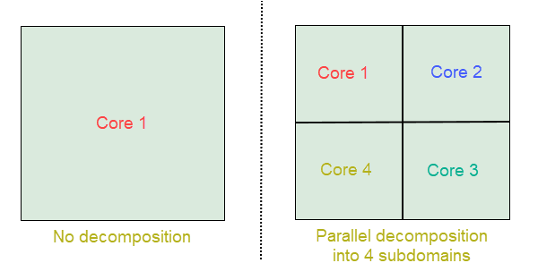
On the left, the simulation of the whole domain is run on just 1 core while on the right the domain is decomposed into 4 equal domains using a decomposition algorithm. The simulation for each domain will now be run simultaneously and the results will be communicated across the domain boundaries to give a final result for the complete domain.
Users with the Community plan have access up to 16 cores, with the Academic plan up to 32 cores, and with the Professional plan up to 192 cores. Selecting more cores will speed up the simulation process but will also burn more core hours. If unsure, choose Automatic, as this option assigns cores in the most economical manner.
When explicitly selecting a machine size, SimScale will attempt to run the simulation on a machine with the required number of processors. Based on availability, a different machine size may be assigned.
Read what core hours are and how they can be managed here.
Maximum Runtime
Here, the maximum time limit can be set in real time after which the simulation will be terminated automatically irrespective of the value set under End time. This setting is important since it helps to control time expenses, especially during the initial iterations.
Potential Flow Initialization
Potential flow initialization works by solving a pressure equation given the velocity initial and boundary conditions, which often provides better initial conditions for the simulation. Toggle-on this setting to accelerate convergence and improve stability during initial time steps if you are experiencing these problems.
Decompose Algorithm
The algorithm to decompose your simulation domain can be specified here. Three algorithms are available viz. Scotch, Hierarchical, and Simple.
- Scotch: The Scotch decomposition algorithm tries to minimize the number of boundaries between the decomposed domains/processors. Fewer boundaries mean reduced required communication between the processors and thus faster simulation. No additional input is required.
Important
SimScale advises its users to always keep the decomposition setting to the default Scotch as this is the most efficient algorithm.
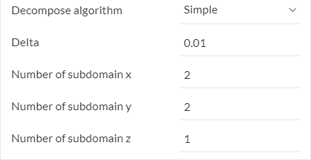
- Simple: It splits the geometric domain depending on the number of subdomains specified in each spatial direction. For example, when a configuration of (2,2,1) is specified for (x,y,z) direction. This is shown in Figure 3.
The additional parameter Delta is defined as cell skew factor. It represents the cell skewness allowed at the subdomain boundaries and is usually kept below 10\(^{-2}\).
- Hierarchical: It acts similarly to the Simple algorithm although with an additional facility of specifying the order of decomposition. A total of six combinations are available viz. XYZ, XZY, YXZ, YZX, ZXY, ZYX.
Important
It is important to note that the number of subdomains should match with the number of assigned cores (see Number of processors above) otherwise the Workbench might throw a validation error.
Last updated: July 14th, 2025
Did this article solve your issue?
How can we do better?
We appreciate and value your feedback.


