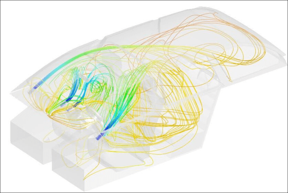
Convective Heat Transfer Analysis
Convective heat transfer analysis can be used in cases where temperature changes in the fluid lead to changes in density. As a result, the fluid circulates under the influence of gravity. The effectiveness of this heat transfer is quantified by the Nusselt number.
Creating a Convective Heat Transfer Analysis
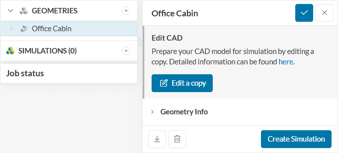
To create a convective heat transfer analysis, the first step is to select the desired geometry and then click on ‘Create Simulation‘:
Afterward, a window with available analysis types appears as follows:
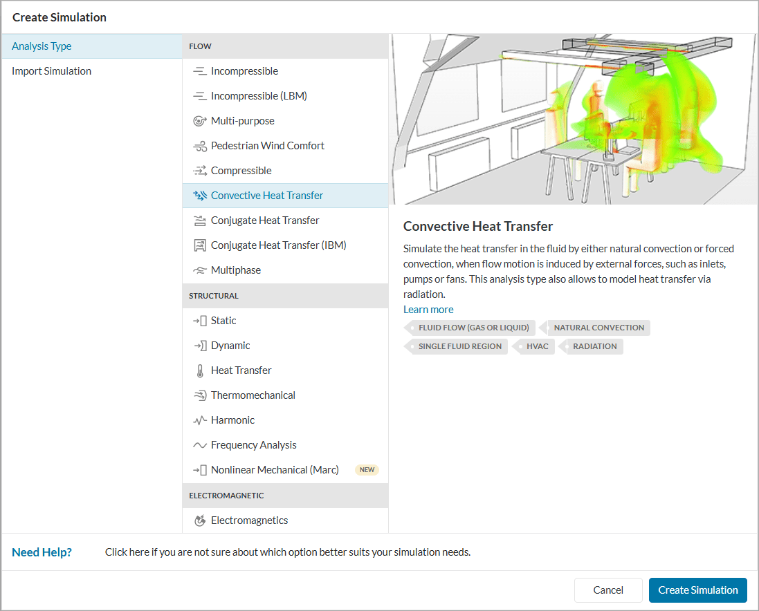
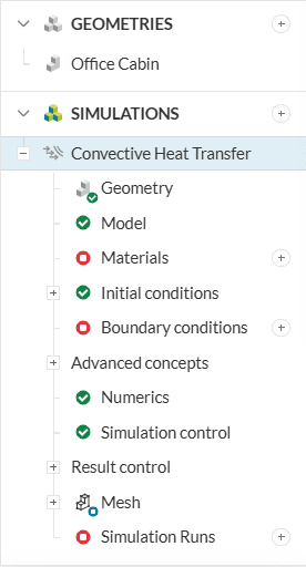
Choose the ‘Convective Heat Transfer’ type from the list and confirm your choice by clicking the ‘Create Simulation‘ button. The following simulation tree with the corresponding settings should appear:
Global Settings
To access the global settings, click on ‘convective heat transfer‘ in the simulation tree. In there, users can configure a series of parameters, namely:
- Toggle compressible on or off;
- Enable or disable radiation;
- Choose the turbulence model;
- Select a steady-state or transient analysis;
- Define the number of passive species being modeled.
For more information about each one of these entries, visit the global settings page.
Geometry
The geometry tab contains the CAD model used for the simulation. Details of CAD handling are described in the pre-processing section.
Important
For convective heat transfer simulations, the solid parts should not be in the domain. Only the fluid domain is necessary.
In SimScale, it’s possible to use flow volume extraction operations to create a flow region and remove the solid parts from the domain.
Alternatively, it’s also possible to create the flow domain in your local CAD software.
Find more details on CAD preparation and upload here.
Model
Under the model, gravity can be defined. If any passive species are being modeled, their diffusion coefficient can also be specified. Lastly, in case LES Smagorinsky or LES Spalart-Allmaras have been set as a turbulence model, their cutoff length can also be configured.
Find further information about the model tab here.
Materials
In the Materials tab, users should specify a fluid for the domain. For more information, please check the relevant documentation page for materials.
Initial Conditions
Initial conditions define the values which the solutions fields will be initialized with. They play a vital role in the stability and computing time of the simulation.
For a convective heat transfer analysis, the velocity, temperature, pressure, and passive scalar fields can either be initialized uniformly or separately via subdomains for each region.
For a complete list of parameters and initialization methods, check out this page.
Important
It is recommended to set the initial conditions close to the expected solution to avoid potential convergence problems.
Boundary Conditions
Boundary conditions define the external input parameters for the simulation. For a complete list of boundary conditions and a description of how they work, make sure to check this page.
Some boundary conditions available in convective heat transfer simulations are supported in parametric experiments. Find an overview of parametric studies in this article.
Important
In case no boundary conditions are assigned to a face, by default it will receive a no-slip wall boundary condition with adiabatic condition (zero gradient) for temperature.
Furthermore, if radiation is enabled, these faces will also be modeled as grey bodies with 0.9 emissivity.
Advanced Concepts
Under advanced concepts, you will find additional setup options, such as rotating zones, power sources, momentum sources, porous media, and passive scalar sources. Visit this dedicated page for more information.
Moreover, momentum sources, power sources, and rotating zones are supported in parametric experiments. Please visit this article for more details.
Note
It’s not possible to create rotating zones if radiation is enabled.
Numerics
Numerical settings play an important role in the simulation configuration. When they are set correctly, they enhance the stability and robustness of the simulation. In most cases, the standard settings should be acceptable, and should not be changed without reason. Find further information here.
Note
SimScale uses its own version of OpenFOAM® solvers developed in-house.
Simulation Control
The simulation control settings define the general controls over the simulation. In this tab, a series of variables can be set. For example, the end time and maximum runtime for the simulation can be defined.
For a complete overview of the parameters and their meaning, check this page.
Result Control
Result control allows users to define additional simulation result outputs. These monitors are helpful to assess the convergence of a simulation. Amongst the available result controls, we have probe points and area averages.
Find more details about result controls here.
Mesh
Meshing is the discretization of the simulation domain. It essentially means to split up a large problem into multiple smaller mathematical problems.
For a convective heat transfer analysis, the standard, hex-dominant, and hex-dominant parametric algorithms are available. For more information about meshes, make sure to check the dedicated page.
Example Projects
- User Guide: Thermal Comfort in a Theater Room
- Tutorial: HVAC Simulation in an Office Environment
- Thermal Comfort in a Warehouse
Last updated: March 25th, 2026
Did this article solve your issue?
How can we do better?
We appreciate and value your feedback.


