Incompressible LBM (Lattice Boltzmann Method) Analysis
The Incompressible LBM analysis type is used to run large transient external aerodynamics simulations when the Mach number is < 0.3 and where the geometry usually involves large domains.
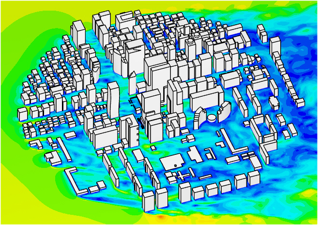
It is a GPU-based solver using the lattice Boltzmann method (LBM), developed by Numeric Systems GmbH, Pacefish®\(^1\). It has the ability to run on multiple GPUs in parallel giving highly accurate results for transient simulations at running times reduced from weeks and days to hours and minutes.
Within SimScale, one can effortlessly set up an incompressible LBM simulation with the steps described below.
Creating an Incompressible LBM Analysis
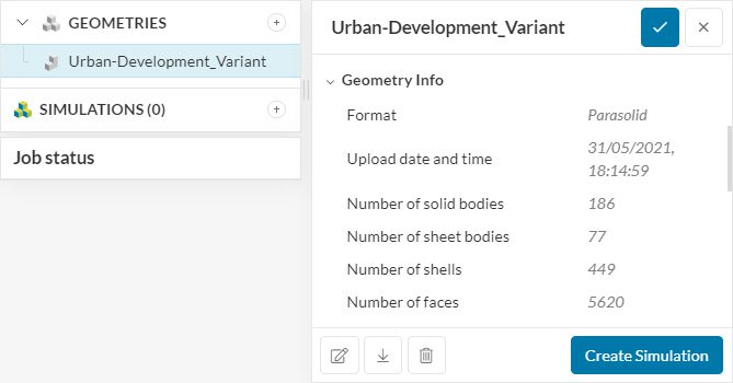
To create an Incompressible (LBM) analysis, first, select the desired geometry and click on ‘Create Simulation’:
Next, a window with a list of several analysis types supported in SimScale will be displayed:
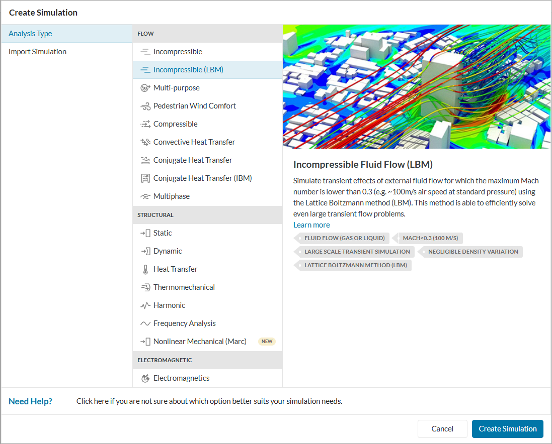
Specialized analysis type
Incompressible (LBM) is a specialized analysis type restricted to users with a paid plan. For more details please visit our product & pricing page or contact sales.
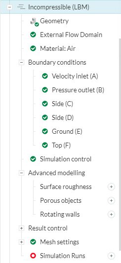
Choose ‘Incompressible (LBM)’ analysis type and click on ‘Create Simulation’. This will lead to the Workbench with the following simulation tree and the respective settings:
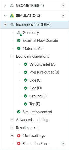
Global Settings
To access the global settings, click on ‘Incompressible (LBM)’ in the simulation tree. Here you can define the turbulence model that needs to be applied for the simulation. A choice between RANS, LES, and DES turbulence models is available.
Detailed information about each of these turbulence models can be found here.
Geometry
The Geometry section allows you to view and select the CAD model required for the simulation. It is important that the CAD model is well prepared to avoid any meshing or simulation-related errors. Find more details on CAD preparation and upload here.
Did you know?
While uploading your CAD model for LBM or wind comfort simulations it is recommended to toggle on ‘Optimize for LBM / PWC’.
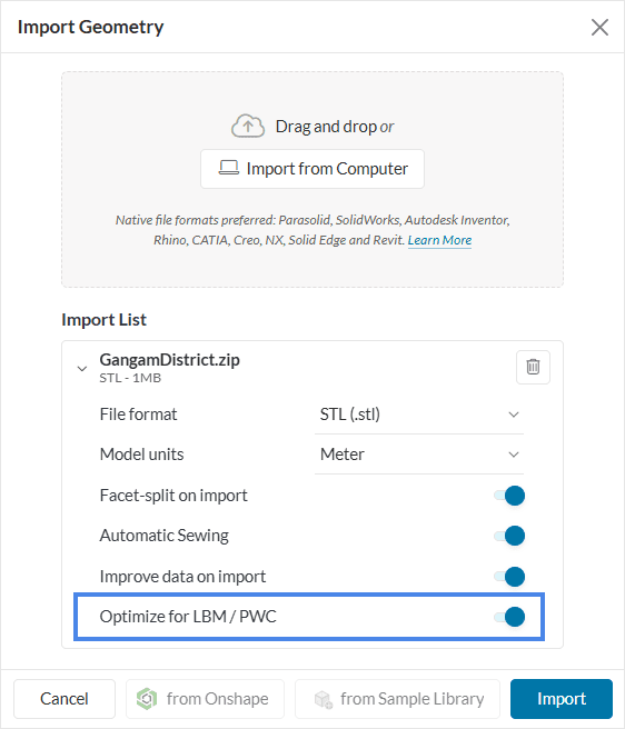
This option allows you to import a *.stl file that is optimized for the incompressible LBM and wind comfort analysis types. It leaves out complex import steps like sewing and cleanup that are not required by the LBM solver and therefore also allows to import big and complex models fast.
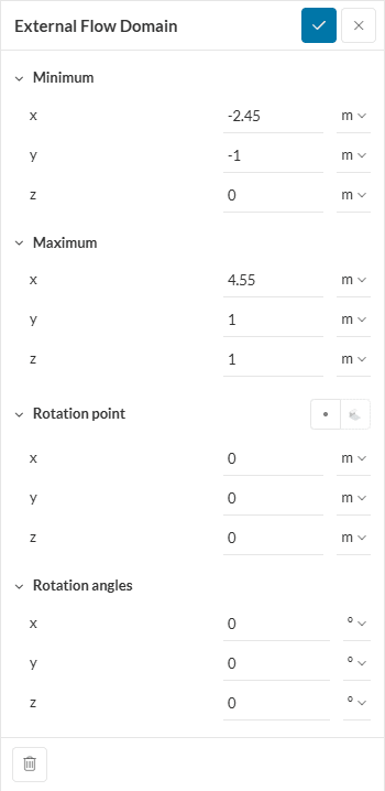
External Flow Domain
Here you can define the cuboidal flow domain that acts as a virtual wind tunnel to perform the fluid flow simulation. You need to define the following parameters:
- Minimum: The minimum values for x-, y-, and z-coordinates
- Maximum: The maximum values for x-, y-, and z-coordinates
- Rotation point: The point about which the flow domain can be rotated. This point can also be picked from the viewer.
- Rotation angles: The angles about x-, y-, and z-axes. Positive values will rotate the domain counterclockwise about the axes (right-hand rule).
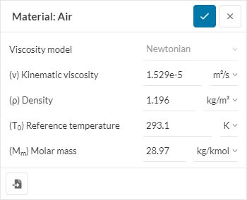
Material: Air
Incompressible LBM simulations currently only support air as the fluid medium. However, air and other gases, at different temperature and pressure conditions, can still be replicated by adjusting the material properties.
Boundary Conditions
Boundary conditions help to add closure to the problem at hand by defining how a system interacts with the environment. Unlike other analysis types, incompressible LBM has a fixed set of boundary conditions assigned to respective faces labeled A through F.
The available boundary conditions and their corresponding faces are listed below:
- Velocity inlet (A)
- Pressure outlet (B)
- Side (C)
- Side (D)
- Ground (E)
- Top (F)
The fundamental boundary conditions used are velocity, pressure, wall, periodic, and atmospheric boundary layer.
Important
All the remaining faces of the CAD model are treated as no-slip walls, that is the velocity is automatically assigned a zero value. The user is not required to assign them separately.
Simulation Control
The Simulation control settings define the general controls over the simulation runtime. The End time, Maximum runtime, and Velocity scaling for the simulation can be defined.
- End time: This represents the time for which the transient effects need to be analyzed (e.g. the physical time).
- Maximum runtime: This is the time value in seconds that decides the maximum time for which the simulation will run on the cloud computing instance. The simulation run is automatically canceled if this value is exceeded. This value is to be used as a safeguard to not run excessively large simulations that could unexpectedly use a large amount of computing quota.
- Velocity scaling: It is used to maintain the stability of the simulation. The default value is 0.1. Read more.
It is advised to read our knowledge base article on controlling simulation time and time steps in LBM for details.
Advanced Modelling
Under Advanced concepts, you will find additional setup options, such as Surface roughness, Porous objects, and Rotating walls. Rotating walls can be applied to cylindrical surfaces which rotate, such as wheels.
Visit this dedicated page for more information.
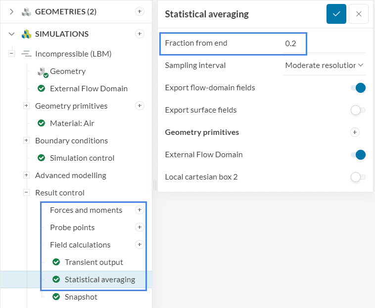
Result Control
The Result Control section allows users to define additional simulation result outputs. It controls how the results will be written meaning the write frequency, location, statistics of the output data, etc.
Find more details about result controls here.
Mesh
Meshing is the process of discretization of the simulation domain. That means we split up a large domain into multiple smaller domains and solve equations for them.
For an incompressible LBM analysis, the meshing is based on the lattice Boltzmann method (LBM) and is quite different from the finite-volume based fluid dynamics analysis types in SimScale. Here a cartesian background mesh is generated, which is composed only of cube elements that are not necessarily aligned with the geometry of the buildings or the terrain.
The mesh characteristics are largely the same as described under the PWC analysis mesh documentation. However, the computation of the region of interest and reference length follows a different logic. Users are strongly advised to read this document before proceeding further.
Depending on whether the mesh settings chosen are automatic or manual the subsequent settings available are as follows:
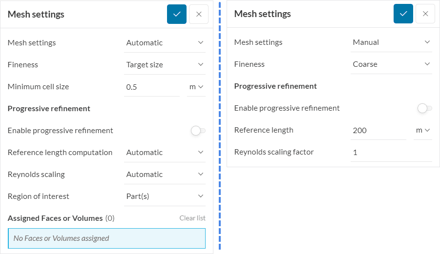
For Automatic mesh settings:
- Fineness: Here, the mesh density can be varied from very coarse to very fine. Alternatively, a minimum target size can be specified under the Target size option. This ensures that the minimum cell size in the region of interest is at most as large as the target cell size (it can be lower). The exact value is reported in the run info. More details about the automatic cell size computation can be found here.
- Reference length computation: This is the longest characteristic length scale of your objects of interest in the simulation. For example, this can include the height of a building or the span of a sports stadium. There’s an option to let the algorithm decide it automatically or enter it manually as a Value.
- Region of interest: The logic for the region of interest is different from the one for the PWC analysis. For incompressible LBM analysis it can be either be a:
- Region defined using a geometry primitive or;
- Part(s) where the user assigns face/s or volume/s directly from the geometry.
For Manual mesh settings:
- Fineness: The mesh density can be varied from very coarse to very fine. The exact value is reported in the run info. The manual cell size computation is different from that of the automatic settings. More details can be found here.
- Reference length: Same as above.
- Reynolds scaling factor: In SimScale, the Reynolds scaling factor (RSF) can be used to apply scaling automatically to a full-scale geometry. This is usually required when tests include scaled versions of buildings or planes in subsonic flows. For more information click here.
The Enable Progressive Refinement option, which is available for both manual and automatic mesh workflows, will be covered in the next section.
Progressive Refinement
The progressive refinement option for LBM simulations allows users to greatly speed up their simulations (usually by 35-45%) while reducing the consumption of computational quota and without significant impact in the results.
During the early stages of a LBM simulation, the flow field needs to develop through the domain, since the initial condition is uniform velocity equal to zero. As such, the intention is to develop the flow field quickly using a coarser mesh, and eventually transition to a fully refined mesh towards the end of the simulation run.
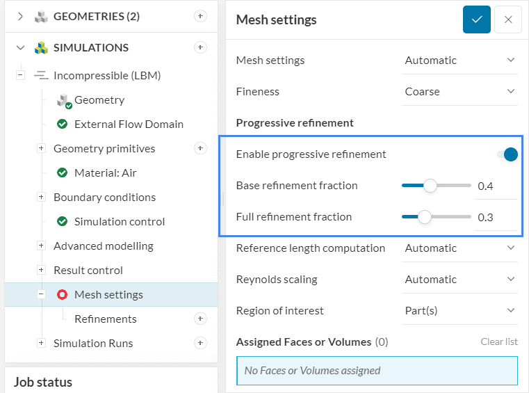
When using progressive refinement, the early stages of the LBM simulation will be run using a base mesh that is two levels of refinement coarser than what the user initially prescribed in the mesh setup. This base refinement mesh will be used from the beginning of the simulation up to the Base refinement fraction defined by the user. As such, the default setting of 0.4 indicates that the base mesh will be used during the first 40% of the simulation run.
The Full refinement fraction indicates the percentage of the simulation run that will be performed with the fully refined mesh. The default setting of 0.3 indicates that the last 30% of the simulation will be performed with the fully refined mesh.
In the interval between base and fully refined meshes, a progressive mesh size transition will take place. After the fully refined mesh starts getting used, it is recommended that the user waits at least 5% of simulation progression before starting to use the results for the transient and statistical result outputs.
With that in mind, the Full refinement factor should be at least 0.05 greater than the Fraction from end defined for result controls.
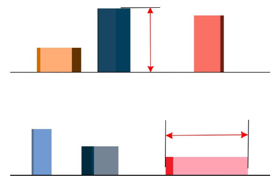
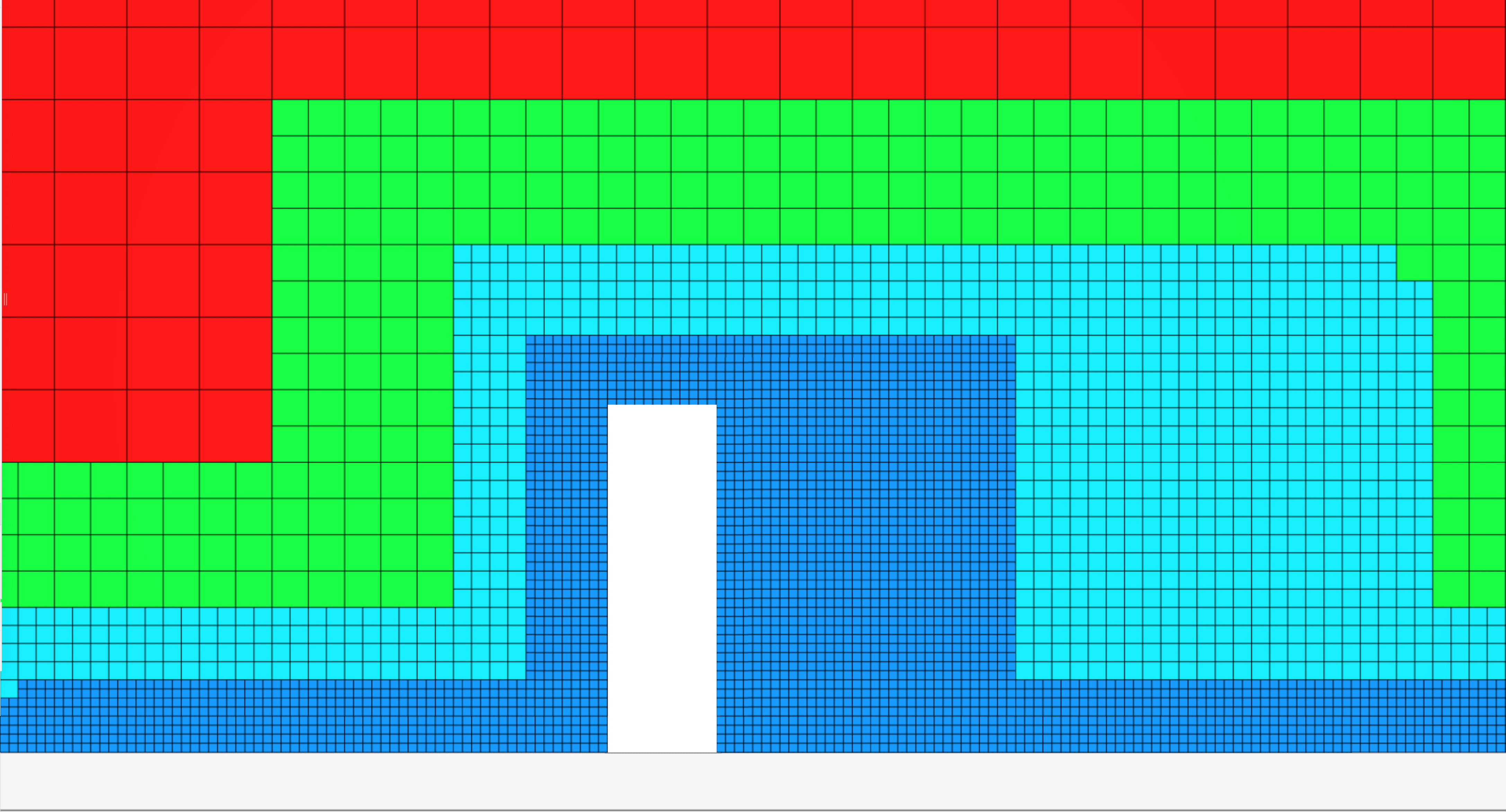
The images below show a comparison between a fully refined mesh and meshes that are 1 and 2 levels coarser, using a simple building geometry for reference.
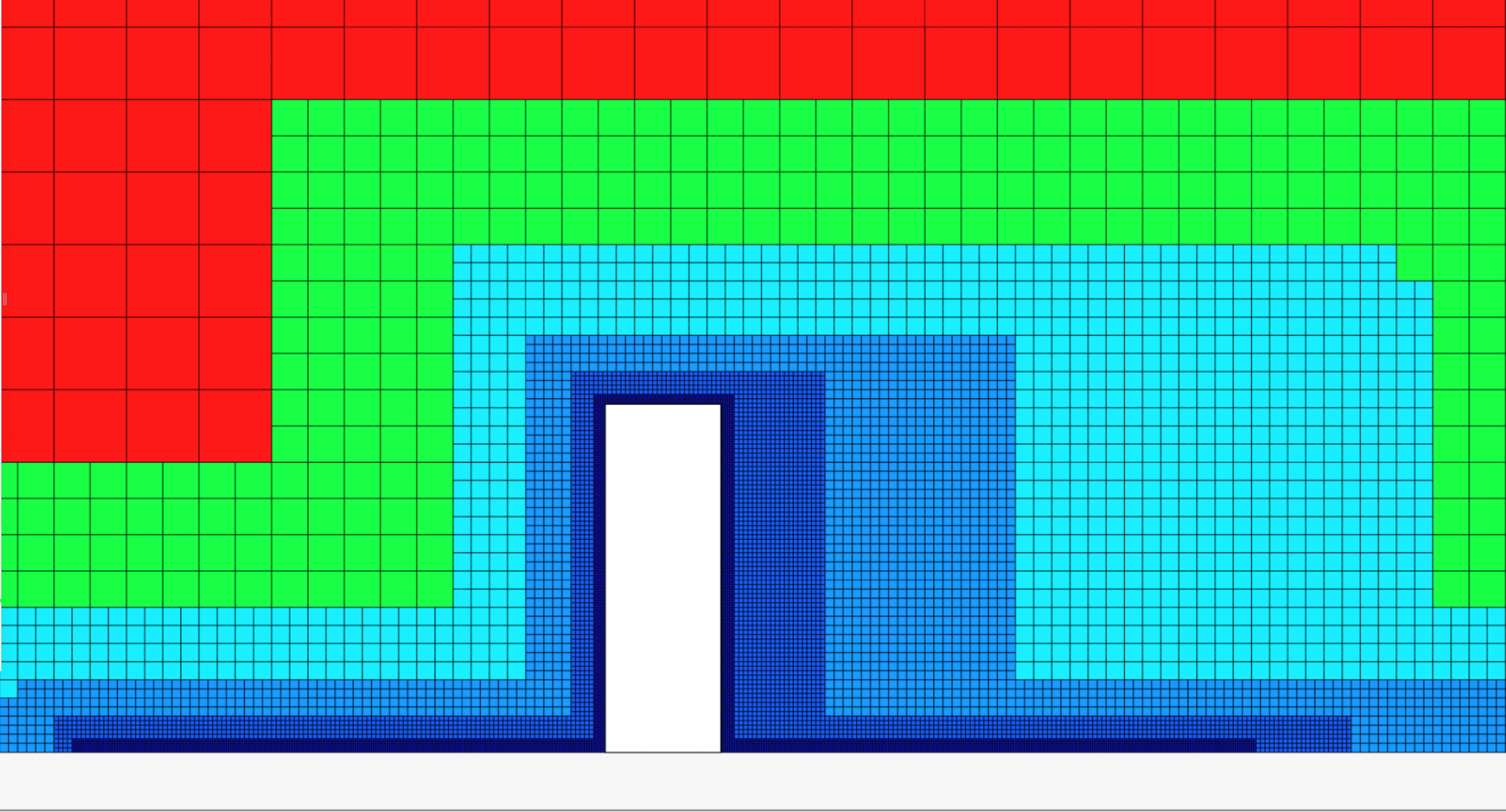
In the scope of progressive refinement, a mesh that is 1 level coarser is generated by coarsening the finest mesh elements of the fully refined mesh:
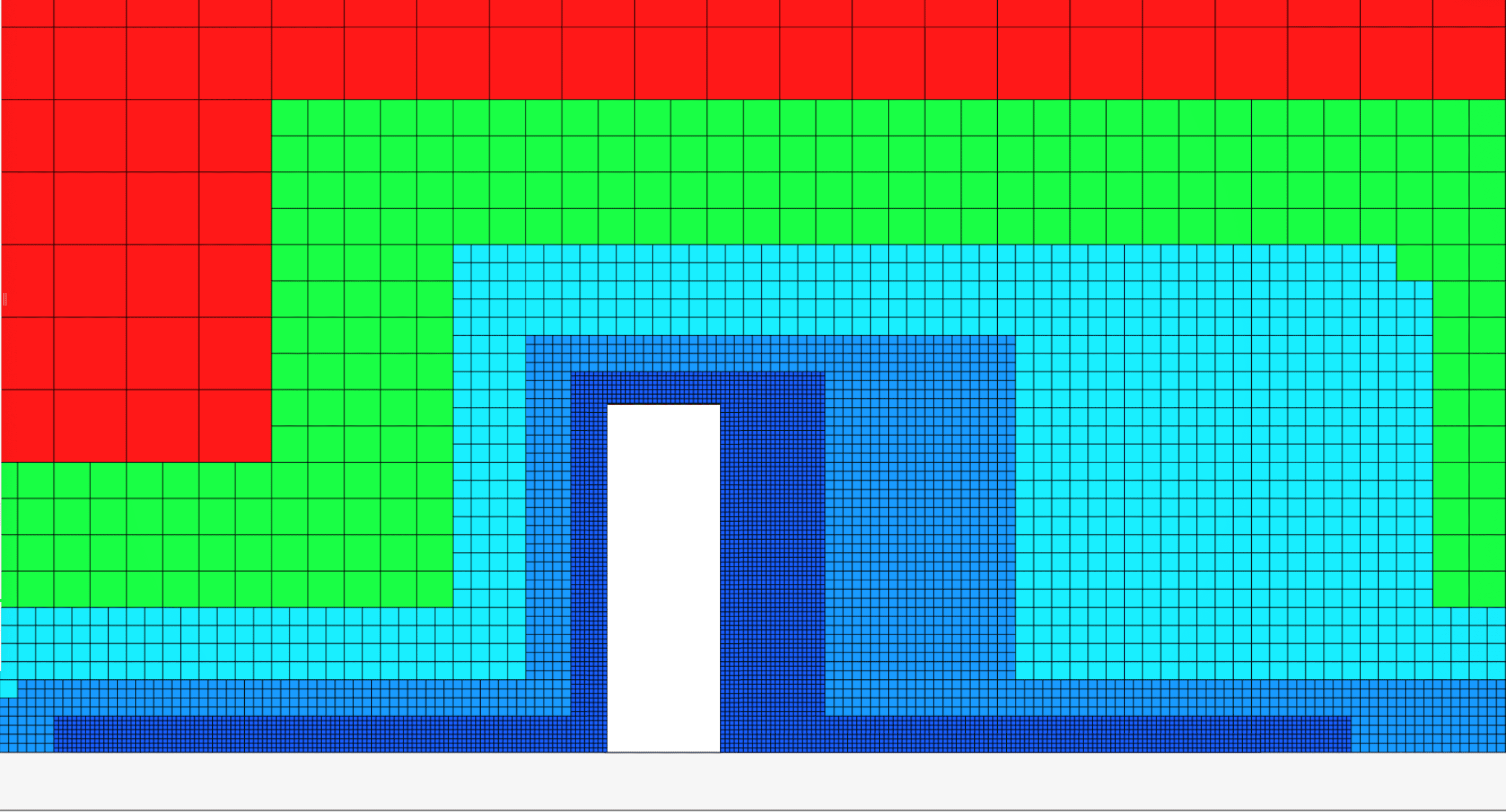
The same happens for the base mesh, yielding the result below:
Local Mesh Refinements
Region Refinement
In case a region between two buildings or a specific open area of interest needs refinement, a region refinement would be best suited. To assign a specific region for mesh refinement, a geometry primitive of type sphere or cartesian box can be locally created using the ‘+’ button and assigned by activating the slider in front of it.
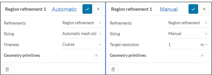
The sizing for the region of interest is managed either automatically by choosing a fineness between very coarse and very fine or by manually setting a target resolution. The parameter Target resolution defines the length scale to which the entire assigned region will be refined.
Surface Refinement
A surface refinement is best suited for cases where a specific building/volume or a set of its surfaces or solids should be refined.
The fineness can be defined analogously to the global mesh sizing from very coarse to very fine. Also, in the same way, as it is done for the global mesh sizing inside the region of interest, the surface refinement will result in a layer of 4-6 cells ranging from the smallest cell size near the surface and gradually increasing with a larger distance from the surface.
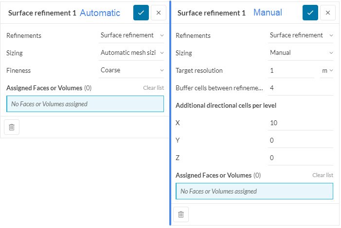
When in manual mode, the user gets to define a minimum number of these buffer layers. Per layer, an additional number of cells in each of the positive x-, y-, z-direction can also be specified.
Related articles
- Blog: GPU-based Solver Using Lattice Boltzmann Method
- Tutorial 1: Pedestrian Comfort Using LBM Solver
- Tutorial 2: Aerodynamics of a Truck
References
Last updated: July 17th, 2025
Did this article solve your issue?
How can we do better?
We appreciate and value your feedback.


