Harmonic

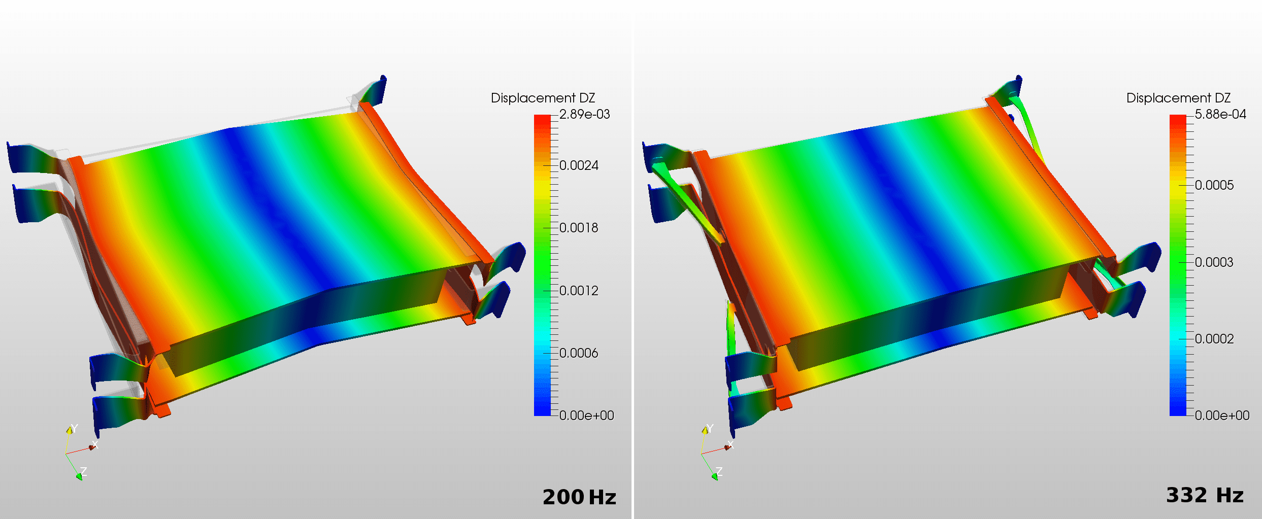
The harmonic analysis type enables the user to simulate the steady-state structural response of solids applied with periodical (sinusoidal) loads. This is similar to a transient dynamic analysis where inertia effects are taken into account, but compared to a transient analysis, the results are not time-dependent but frequency-dependent. Thus, making it possible to compute the response of a structure subjected to vibrating forces or displacements over a frequency spectrum.

This is a linear simulation, therefore one can only use linear elastic materials. However, damping effects can be analyzed.

All linear boundary conditions are available for this simulation type and the loadings can be dependent on the frequency of the excitation.

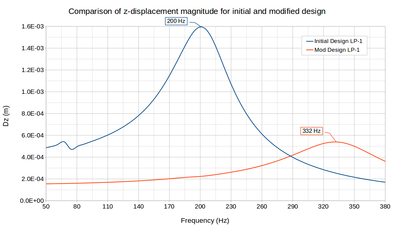
The results of a harmonic simulation are of complex nature and the user can specify how the results are exported in Result control, either as Magnitude and Phase or as Real and Imaginary parts. Under Result control, the user can also place probe points under Point data. One can use this to gather data at specific points which can be used as a comparison against measured data.

Creating a Harmonic Analysis

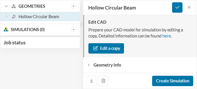
The user can create a harmonic analysis by clicking on the uploaded geometry and then on the ‘Create Simulation’ button.

Afterwards, the user will be able to select a Harmonic analysis from the list of the available simulation types in SimScale.

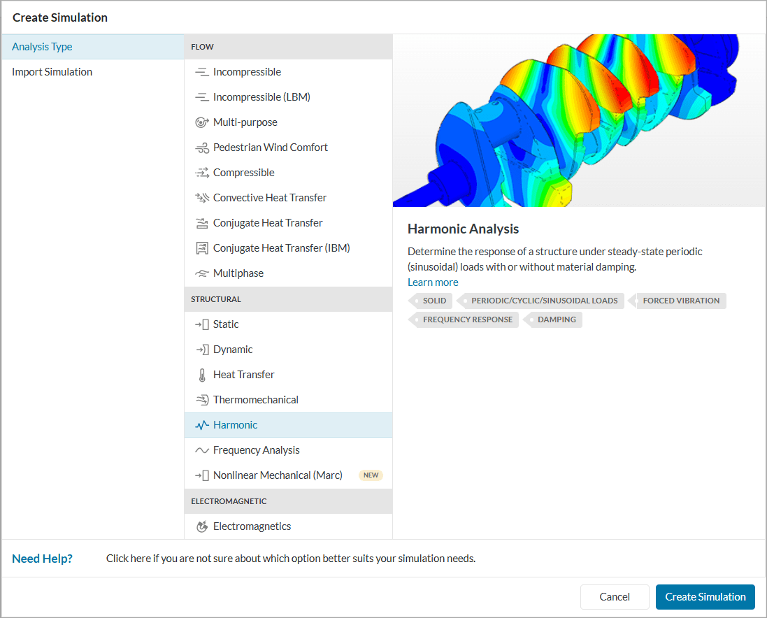
Finally, the user will be able to set up the harmonic analysis simulation by following the necessary steps.

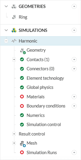
Geometry

This contains information regarding the selected simulation domain. One can read more regarding CAD preparation in the pre-processing section of the documentation.

Contacts

If parts of the model are in contact with each other, SimScale will automatically detect these contacts. However, the user can also create the contacts manually, and choose between three different contact definitions:

• Bonded
• Cyclic symmetry
• Sliding

For more information, refer to the Contacts section of the documentation.

Element Technology

The user can choose the 3D element technology to be implemented. There are two options that can be seen below:

• Standard
• Reduced integration

We recommend using standard for first order elements and reduced integration for second order elements.

Materials

As described before, a harmonic analysis can only use linear elastic materials.

The user can define the material properties of one or multiple solids, however, depending on the law of the material, they may need to define different properties. In addition to Young’s modulus and Poisson’s ratio, the density of the material is also necessary.

In addition, there are two damping models available for harmonic analysis:

• Hysteretic damping
• Rayleigh damping

For more information, refer to the Materials section of the documentation.

Boundary Condition

As described before, all linear boundary conditions are available for harmonic analysis. The user also does not need to consider the sinusoidal application of the boundary conditions as this is done implicitly. One can define a phase angle for each boundary condition which allows the consideration of different phase offsets between each boundary condition.

The boundary conditions can be dependent on the excitation frequency, where the values change over the frequency range. For vector-valued boundary conditions, this can be done with the scaling parameter, which can be defined as a scalar, or as a function of frequency or as table data.

The boundary conditions are of two kinds, constraints and load.

• Constraints (Displacement boundary conditions):
  • Fixed Value
  • Remote Displacement
  • Symmetry
• Load (Force boundary conditions):
  • Pressure
  • Force
  • Remote force
  • Surface load
  • Volume load
  • Nodal load
  • Centrifugal force

For more information, refer to the Boundary Conditions section of the documentation.

Numerics

Under Numerics, the user can set the solver equation for the simulation. SimScale incorporates the finite element solver Code_Aster which have three direct linear solvers for harmonic analysis:

• Multfront
• MUMPS
• LDLT

For more information, the refer to the Numerics section of the documentation.

Simulation Control

The user can define a frequency range for the simulation, either as a single frequency or a list of frequencies. The list of frequencies is defined with the start frequency, the frequency stepping length and the end frequency.

One will also be able to define the number of processors (CPU) assigned to the simulation and the maximum allowable runtime for the simulation.

For more information, refer to the Simulation Control section of the documentation.

Result Control

Here, the data that will be exported can be defined. The user can define the solution fields that will be calculated and exported under Solution Fields and define measurement points under Point data.

Solution fields

The user can add or exclude solution fields that will be calculated and exported. They can also choose between Magnitude and Phase or Real and Imaginary as the representation of complex numbers for each solution field.

Point data

Specific measurement points can be defined to monitor the structural response of the model with geometry primitives. The user can also control the solution field, the vector component, and the representation of the complex numbers that will be exported for each specific point.

For more information, refer to the Result Control section of the documentation.

Mesh

A first or second order mesh can be used to discretize the geometry. The user will be able to define how the mesh will be refined at this step.

After the mesh has been generated, information regarding the mesh will be provided and the mesh quality will be observed.

For more information, refer to the Meshing section of the documentation.

Last updated: June 30th, 2020