Model
Under the Model tab, additional parameters that define the physics of the simulation are defined.
For convenience, the setup parameters will be divided into two main categories: computational fluid dynamics (CFD) and finite element analysis (FEA).
Computational Fluid Dynamics
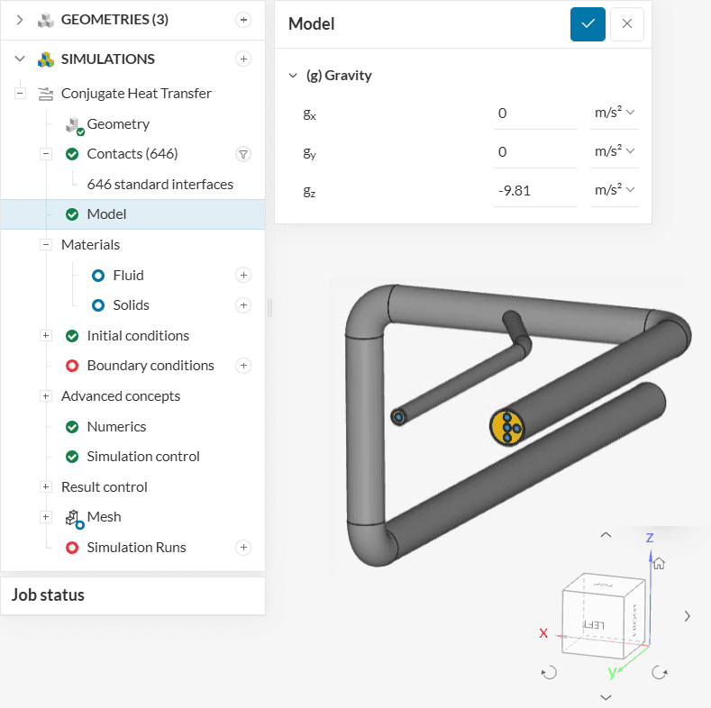
Gravity
For fluid flow analysis, gravity is defined via a vector. The global coordinate system, represented by the orientation cube, applies for the gravity direction. The vector coordinates \(g_x\), \( g_y\), and \(g_z\) represent the x, y, and z directions.
Please note that incompressible simulations do not require a definition for gravity, as it is a single-phase analysis where buoyancy effects are not present.
Passive Species
In case passive species are defined in the global settings, the Turbulent Schmidt number and the Diffusion coefficient can be specified in the model section.
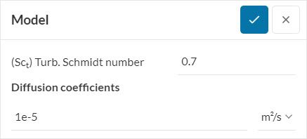
\((Sc_t)\) Turb. Schmidt number
The turbulent Schmidt number represents the ratio between the turbulent transport of momentum and the turbulent transport of mass. In SimScale, it will play a role in the transport of the passive species throughout the domain.
It is important to note that the turbulent Schmidt number is characteristic of the flow, and not the fluid. Typical values for this parameter range from 0.5 to 1.3. In case you are not familiar with the flow that you are analyzing, it is recommended to maintain the default value of 0.7 for all passive species.
Diffusion coefficients
The Diffusion coefficient is a parameter highlighted in Fick’s First Law:
$$J = -D \frac {d\psi}{dx}$$
where:
\(J\) is the diffusion flux;
\(D\) is the diffusion coefficient;
\(\frac {d\psi}{dx}\) is the spatial gradient of the substance’s concentration.
Therefore, the diffusion coefficient is the factor of proportionality between the flux and the spatial gradient of a diffusing species\(^1\). It is possible to find diffusion coefficients for a pair of substances on journal publications, as well as engineering websites such as the Engineering ToolBox\(^2\).
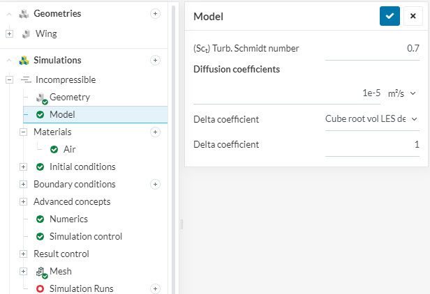
Delta Coefficient
This setting is available for the OPENFOAM® solvers whenever a large eddy simulation (LES) turbulence model is chosen (see Figure 1).
In an LES simulation, only the large eddies are fully resolved. Resolving eddies of all scales results in an enormous computational effort. For this reason, the Delta coefficient is used as a filter for the subgrid-scale.
The Delta coefficient will be related to the local cell size. The smaller eddies that are filtered out are modeled using a RANS approach. Meanwhile, large eddies continue to be fully resolved.
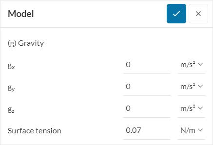
Surface Tension
For a multiphase analysis, the surface tension between the phases can be defined here. It is possible to find the surface tension values for various fluids in online sources such as the Engineering ToolBox\(^2\).
Finite Element Analysis
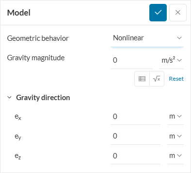
Geometric Behavior
There are two valid settings for Geometric Behavior: Linear and Nonlinear.
When choosing a Linear behavior, the numerical model of the solid parts is not updated as the simulation progresses. Therefore, during the entire simulation, the loads, deformations, and physics will take into account the initial state of the geometry. For this reason, a linear behavior is only a good approximation when the model undergoes small deformations and small rotations.
The Nonlinear option is a better choice when large rotations and deformations are expected. The mathematical model is updated after each step, allowing a precise computation of the results throughout the simulation.
The geometric behavior definition is only necessary in the following cases:
- Nonlinear static simulations
- Dynamic studies
- Transient nonlinear thermomechanical simulations
Gravity
In the case of structural analysis, gravity magnitude and direction must be specified separately. Furthermore, the gravity magnitude can also be defined as a function of time via table and formula input. Please note that aligning the model with the global coordinates is always recommended, as it is easier to set up gravity and boundary conditions.
If your model needs to remain misaligned with the global coordinate axis, it is still possible to set up gravity accordingly. For example, the image below shows the gravity definition for the gravity vector when it’s 30 degrees off the y-axis:
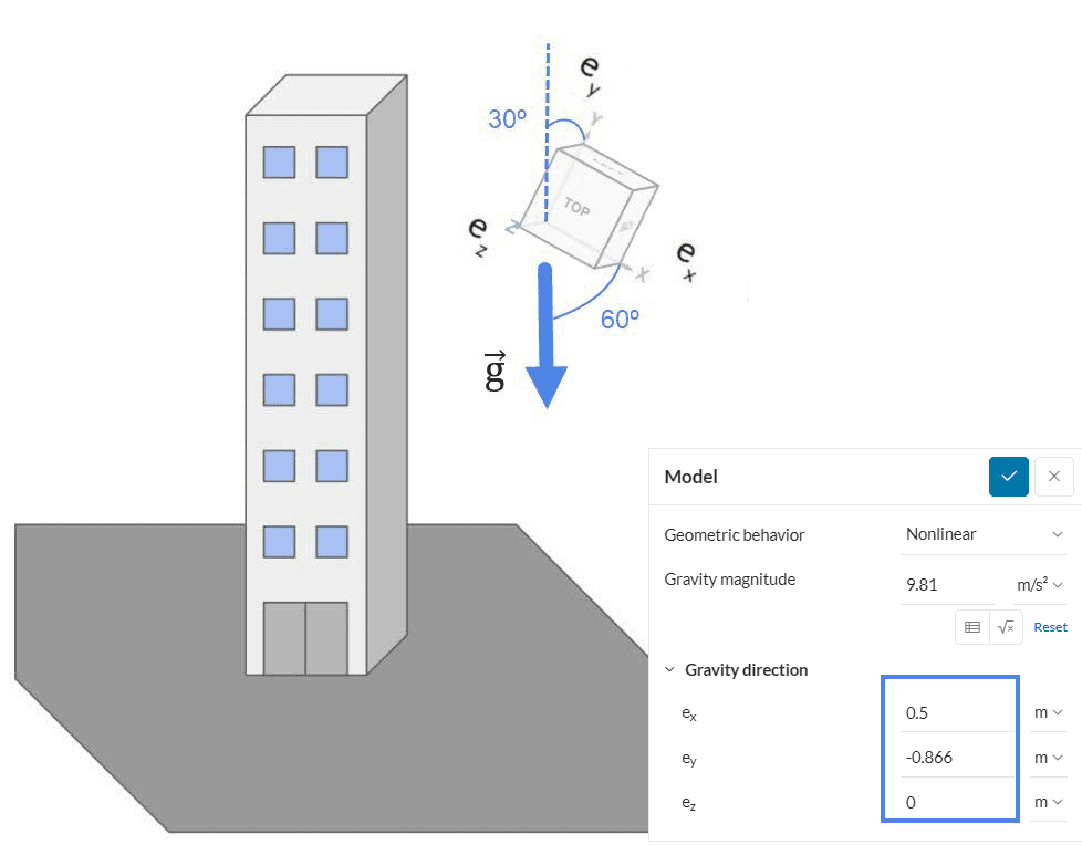
In this case, the vector coordinates are calculated as below:
\(e_x = sin (30 deg) = cos (60 deg) = 0.5 \tag{1}\)
\(e_y = – cos (30 deg) = – sin (60 deg) = – 0.86602540378 \tag{2}\)
\(e_z = 0 \tag{3}\)
References
Last updated: June 4th, 2025
Did this article solve your issue?
How can we do better?
We appreciate and value your feedback.


