K-Omega Turbulence Models
SimScale allows different methods to model the turbulent effects appearing in a CFD simulation. The SimScale CFD solver uses its in-house version of the widely accepted industry standard turbulence models. This document sheds light on the popular k-omega turbulence models.
Overview
The Reynolds-averaged Navier Stokes (RANS) equation in tensor form\(^1\) can be written as:
$$ {\frac{\partial (\rho U_i)}{\partial t}} + {\frac{\partial (\rho U_iU_j)}{\partial x_j}} = -\frac{\partial P}{\partial x_i} + {\frac{\partial}{\partial x _ j}\left[\mu\left(\frac{\partial U _ i}{\partial x _ j} + \frac{\partial U _ j}{\partial x _ i}\right) – \rho \overline{{u_i}'{u_j}’}\right]} \tag{1} $$
where,
- \(U\) = mean flow velocity
- \(u’\) = velocity fluctuations due to turbulence
- \(\mu\) = molecular viscosity
- \(-\rho \overline{{u_i}'{u_j}’}\) = Reynolds Stress term
The Reynolds averaging process results in an additional stress term – Reynolds Stress. To solve the RANS equations we need to express the Reynolds stress in terms of mean flow quantities.
The solution for the Reynolds stress term is given by the Eddy viscosity hypothesis/ Boussinesq hypothesis\(^1\) as
$$-\rho \overline{{u_i}'{u_j}’} = \mu_t\left(\frac{\partial U_i}{\partial x_j}+ \frac{\partial U_j}{\partial x_i} -\frac{2}{3}\frac{\partial U_k}{\partial x_k} \delta_{ij} \right) -\frac{2}{3} \rho k \delta_{ij} \tag{2}$$
where,
- \(\mu_t\) = turbulent or eddy viscosity
- \(\delta_{ij}\) = Kronecker Delta
$$ \delta_{ij} =
\begin{cases}
1, & \text{if $i=j$ \(\to\) Normal stress component} \\[2ex]
0, & \text{if $i \neq j$ \(\to\) Shear stress component}
\end{cases}$$
Equation 2 is a combined equation for the shear and normal components of Reynolds stresses. Observing equation 2 we realize that once we solve for the turbulent viscosity \((\mu_t)\) we can solve the RANS equation 1.
Hence, the difference between different turbulent models is the methodology to calculate turbulent viscosity.
K-Omega Turbulence Models
The k-omega (\(k-\omega\)) turbulence model is one of the most commonly used models to capture the effect of turbulent flow conditions. It belongs to the Reynolds-averaged Navier-Stokes (RANS) family of turbulence models where all the effects of turbulence are modeled.
It is a two-equation model. That means in addition to the conservation equations, it solves two transport equations (PDEs), which account for the history effects like convection and diffusion of turbulent energy. The two transported variables are turbulent kinetic energy (\(k\)), which determines the energy in turbulence, and specific turbulent dissipation rate (\(\omega\)), which determines the rate of dissipation per unit turbulent kinetic energy. \(\omega\) is also referred to as the scale of turbulence.
If you read about the \(k-\epsilon\) turbulence model you will realize that \(\epsilon\) and \(\omega\) essentially represent the dissipation of turbulent kinetic energy \((k)\).
The relation between dissipation rate \((\epsilon)\) and specific dissipation rate \((\omega)\) is given by
$$ \epsilon = C_{\mu}k \omega \tag{3}$$
where, \(C_\mu\) = 0.09
Different variations of the k-omega model exist such as Standard k-omega, k-omega BST, k-omega SST, etc. each with certain modifications to perform better under certain fluid flow conditions. In SimScale, the standard k-omega and k-omega SST versions are available.
Standard K-Omega Model
Transport Equations for the Turbulence Variables
The transport equation for turbulent kinetic energy \((k)\) is given by\(^2\)
$$ {\frac{\partial (\rho k)}{\partial t}} + {\frac{\partial (\rho U_ik)}{\partial x_i}} = {\frac{\partial}{\partial x _j}}\left[\left(\mu+\frac{\mu_t}{\sigma_k} \right){\frac{\partial k}{\partial x_j}}\right] + P_k + P_b -\rho \epsilon +S_k \tag{4} $$
where,
- \(P_k\) = production of turbulent kinetic energy (TKE) due to mean velocity shear
- \(P_b\) = production of TKE due to buoyancy
- \(S_k\) = user-defined source
- \(\sigma_k\) = turbulent Prandtl number for \(k\)
The transport equation for the turbulent dissipation rate \((\epsilon)\) is given by\(^2\)
$$ {\frac{\partial (\rho \epsilon)}{\partial t}} + {\frac{\partial (\rho U_i \epsilon)}{\partial x_i}} = {\frac{\partial}{\partial x _j}}\left[\left(\mu+\frac{\mu_t}{\sigma_\epsilon} \right){\frac{\partial \epsilon}{\partial x_j}}\right] + C_1 \frac{\epsilon}{k}(P_k +C_3P_b) -C_2 \rho \frac{\epsilon^2}{k} + S_\epsilon \tag{5} $$
where,
- \(C_1, C_2, C_3, C_\mu\) are model coefficients that vary within \(k-\epsilon\) turbulence models
- \(S_\epsilon\) = user-defined source
- \(\sigma_\epsilon\) = turbulent Prandtl number for \(\epsilon\)
Substituting equation 3 in equation 5 gives us
$$ {\frac{\partial (\rho \epsilon)}{\partial t}} + {\frac{\partial (\rho U_i \epsilon)}{\partial x_i}} = {\frac{\partial}{\partial x _j}}\left[\left(\mu+\frac{\mu_t}{\sigma_\epsilon} \right){\frac{\partial \epsilon}{\partial x_j}}\right] + \frac{\gamma}{\nu_t}P_k -\beta\rho\omega^2 + \underbrace{\frac{2\rho{\sigma_{\omega}}^2}{\omega} \Delta k: \Delta \omega}_{Additional\ term} \tag{6}$$
where,
$$\Delta k: \Delta \omega = \frac{\partial k}{\partial x_j}\frac{\partial \omega}{\partial x_j}$$
The term,
$$\frac{2\rho{\sigma_{\omega}}^2}{\omega} \Delta k: \Delta \omega$$
is an additional term appearing as a part of substitution. Without this term we can call equation 6 as the transport equation for the specific dissipation rate \((\omega)\).
Difference between \(k-\epsilon\) and \(k-\omega\) turbulence models
Since \(\epsilon\) and \(\omega\) essentially represent turbulent dissipation the real difference between \(k-\epsilon\) and \(k-\omega\) models is the empirical coefficients appearing in the equations (\(\sigma_k, \sigma_\epsilon, \beta ……)\)
Modeling Turbulent Viscosity
As explained in the K-Epsilon Turbulence Models documentation, older turbulence models used a mixing length approach to solve for the turbulent (Eddy) viscosity. The \(k-\epsilon\) turbulence models solve directly for the turbulence dissipation rate instead.
Since epsilon and omega both represent the dissipation of turbulent kinetic energy we can solve for the transport of either epsilon or omega and simply convert using equation 3.
The turbulent energy \(k\) is given by:
$$k=\frac { 3 }{ 2 } { \left( UI \right) }^{ 2 }\tag{7}$$
where \(U\) is the mean flow velocity and \(I\) is the turbulence intensity.
The turbulence intensity gives the level of turbulence and can be defined as follows:
$$I = \frac { u’ }{ U }\tag{8}$$
where \(u’\) is the root-mean-square of the turbulent velocity fluctuations given as:
$$u’ = \sqrt { \frac { 1 }{ 3 } \left( { { u’ }_{ x } }^{ 2 } + { { u’ }_{ y } }^{ 2 } + { { u’ }_{ z } }^{ 2 } \right) } =\sqrt { \frac { 2 }{ 3 } k }\tag{9}$$
The mean velocity \(U\) can be calculated as follows:
$$U = \sqrt { { { U }_{ x } }^{ 2 }+{ { U }_{ y } }^{ 2 }+{ { U }_{ z } }^{ 2 }}\tag{10}$$
The turbulent dissipation rate can be calculated using the following formula:
$$\omega ={ { C }_{ \mu } }^{ \frac { 3 }{ 4 } }\frac { { k }^{ \frac { 1 }{ 2 } } }{ l }\tag{11}$$
where \({ { C }_{ \mu } }\) is the turbulence model constant, \(l\) is the turbulent length scale.
The turbulence length scale describes the size of large energy-containing eddies in a turbulent flow.
The turbulent viscosity \(\mu_t\) is, thus, calculated as:
$$\mu_{t} = \frac{\rho k}{\omega}\tag{12}$$
Applications
The standard \(k-\omega\) model is a low \(Re\) model, i.e., it can be used for flows with low Reynolds number where the boundary layer is relatively thick and the viscous sublayer can be resolved.
The k-epsilon model uses empirical damping functions in the viscous sub-layer region which were essentially derived for the flat plate boundary layer flows. They are not very accurate in the presence of adverse pressure gradients like in flows past airfoil and turbine blades. K-omega model doesn’t require these damping functions giving a better accuracy.
Thus, the standard \(k-\omega\) model is best used for near-wall treatment. Other advantages include a superior performance for complex boundary layer flows under adverse pressure gradients and separations (e.g., external aerodynamics and turbomachinery).
One drawback of this model is that it is dependent on the free stream values/inlet conditions for the turbulence. For small changes in \(k\) it is known to show large changes in turbulent viscosity and skin friction coefficient causing excessive and early separations and inaccurate capturing of forces on the body\(^2\).
K-Omega SST
The Basis
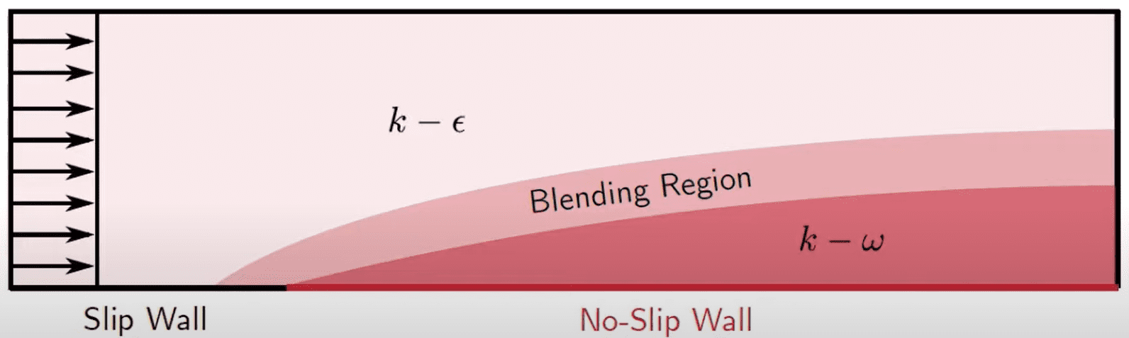
The k-epsilon model tends to show great results in the free stream region and the k-omega model has a good accuracy in the boundary layer region close to the wall. We can combine the advantages of these two turbulence models using a blending function.
One of the drawbacks of the k-omega model is its susceptibility to the free stream values of \(k, \omega,\) and \(\epsilon\). K-epsilon turbulence model on the other hand is not as susceptible and rather robust in those aspects.
Hence, we use a blending function to switch from the k-epsilon model away from the wall (free stream region) to the k-omega model close to the wall.
Transport Equations for the Turbulence Variables
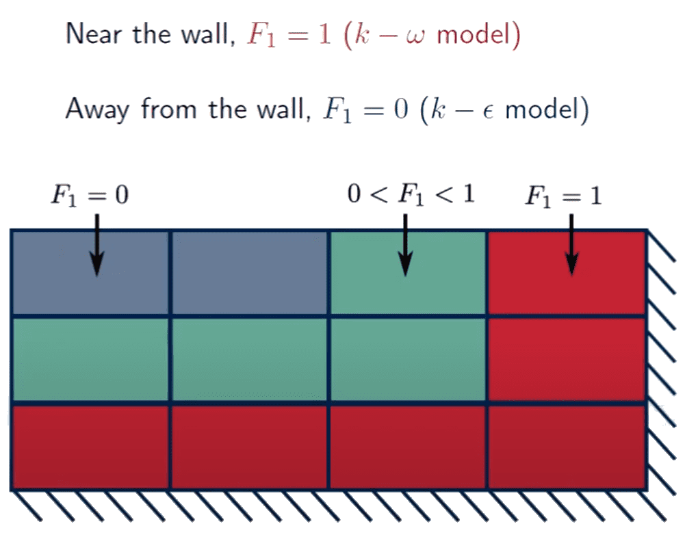
If we multiply the additional term in equation 6 using a function (1- \(F_1\)) the equation now becomes
$$ {\frac{\partial (\rho \epsilon)}{\partial t}} + {\frac{\partial (\rho U_i \epsilon)}{\partial x_i}} = {\frac{\partial}{\partial x _j}}\left[\left(\mu+\frac{\mu_t}{\sigma_\epsilon} \right){\frac{\partial \epsilon}{\partial x_j}}\right] + \frac{\gamma}{\nu_t}P_k -\beta\rho\omega^2 + (1-F_1)\underbrace{\frac{2\rho{\sigma_{\omega}}^2}{\omega} \Delta k: \Delta \omega}_{Additional term} \tag{13}$$
If \(F_1\) is zero the additional term remains and thus equation 13 is the transport equation for \(\epsilon\) representing a \(k-\epsilon\) turbulence model.
If \(F_1\) is 1 the additional term vanishes and thus equation 13 is the transport equation for \(\omega\) representing a \(k-\omega\) turbulence model.
The Blending Function
\(F_1\) is called the Blending function as it effective blends the two turbulence models. Mathematically speaking, it is a hyperbolic function that is used for a smooth transition between the k-omega model and the k-epsilon model. This along with an additional viscosity limiter forms as the basis for the k-omega SST (shear stress transport) model.
Modeling Turbulent Viscosity
The turbulent viscosity \((\mu_t)\) for the k-omega model is calculated as
$$\mu_{t} = \frac{\rho k}{\omega}$$
For the k-omega SST model the turbulent viscosity is calculated as\(^3\)
$$\mu_{t} = \frac{a_1 \rho k}{max(a_1\omega,SF_2)} \tag{14}$$
where,
- \(F_2\) is another blending function
- \(S\) is the magnitude of shear strain
Hence, if \(SF_2\) is larger than \(a_1 \omega\) the viscosity is limited (i.e. reduced) resulting in better agreement with the experimental measurements of separated flows.
Applications
The \(k-\omega\) SST model is the most widely accepted industry standard turbulence model. It provides a better prediction of flow separation than most RANS models and also accounts for its good behavior in adverse pressure gradients. It has the ability to account for the transport of the principal shear stress in adverse pressure gradient boundary layers. It is the most commonly used model in the industry given its high accuracy to expense ratio.
On the negative side, the \(k-\omega\) SST model produces some large turbulence levels in regions with large normal strain, like stagnation regions and regions with strong acceleration. This effect is much less pronounced than with a normal k-epsilon model though.
Inlet Turbulence
To realistically model a given problem, it is important to define the turbulence intensity at the inlets. Here are a few examples of common estimations of the incoming turbulence intensity:
- High-turbulence (between 5% and 20%): Cases with high velocity flow inside complex geometries. Examples: heat exchangers, flow in rotating machinery like fans, engines, etc.
- Medium-turbulence (between 1% and 5%): Flow in not-so-complex geometries or low speed flows. Examples: flow in large pipes, ventilation flows, etc.
- Low-turbulence (well below 1%): Cases with fluids that stand still or highly viscous fluids, very high-quality wind tunnels. Examples: external flow across cars, submarines, aircraft, etc.
Did you know?
The turbulent intensity at the core of a pipe for a fully developed pipe flow can be estimated as follows:
$$I=0.16 { { Re }_{ { d }_{ h } } }^{ -\frac { 1 }{ 8 } }\tag{15}$$
where \({ { Re }_{ { d }_{ h } } }\) is the Reynolds number for a pipe of hydraulic diameter \({ { d }_{ h } }\).
The turbulence length scale in this case is
$$l=0.07{ d }_{ h }\tag{16}$$
Applying K-Omega Model in SimScale
The k-omega turbulence model needs to be chosen at the beginning of the simulation setup inside the global settings panel. This is shown in the figure below:
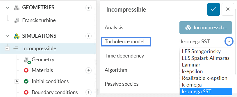
By default, SimScale defines the initial values of turbulence variables \(k\) and \(\omega\) depending on the domain of the problem. If needed, they can be changed under Initial conditions. Further, if the user wants to specifically define the boundary conditions for these turbulence variables, then the Custom boundary condition can be used.
References
- “[CFD] Eddy Viscosity Models for RANS and LES.” Fluid Mechanics 101. February 24, 2021.
- “[CFD] The k-omega Turbulence Model.” Fluid Mechanics 101. June 4, 2020.
- “[CFD] The k – omega SST Turbulence Model.” Fluid Mechanics 101. March 14, 2019.
- Menter, Florian R. “Improved two-equation k-omega turbulence models for aerodynamic flows.”, 1992.
- Wilcox, David C, “Turbulence Modeling for CFD”. Second edition. Anaheim: DCW Industries, pp. 174, 1998.
- https://www.cfd-online.com/Wiki/Turbulence_free-stream_boundary_conditions
Last updated: April 8th, 2025
Did this article solve your issue?
How can we do better?
We appreciate and value your feedback.


