Structural Analysis Numerics
The Numerics panel contains the settings that control the equation solvers for FEA Structural Analysis models. This includes the selection of algorithms, type of residuals and threshold values, maximum number of iterations, time integration schemes, etc. Following is a detailed description of each one of the settings and its effects on the solution process.
The set of default values for these parameters is good enough for most situations, but advanced users can leverage the available options to optimize their solution process, for speed, robustness, and precision.
Linear Equations Solver

Linear equation solvers are algorithms that solve the general linear equation:
$$ Ku=F $$
For the unknowns \(u\), given a matrix of coefficients \(K\) and an independent term \(F\). This type of equation appears naturally in the Finite Elements Method, as a result of the discretization of the continuum. In other words, a set of linear equations appear when changing a domain of continuum variables into the discrete finite elements domain, where the variables are computed at a finite number of points.
Many optimized algorithms have been developed to efficiently solve the general linear equation. The two main families are the direct solvers and the iterative solvers:
- Direct solvers decompose the coefficient matrix into factors by leveraging the matrix properties, and then find the solution by simple operations such as matrix-vector multiplication.
- Iterative solvers start with a guess solution and then implement a process of successive approximations until convergence is reached.
Direct solvers are generally preferred because they are more robust, but they are limited by the number of equations to solve due to their higher memory consumption. For larger models, an iterative solver could be the only option. Also, iterative solvers allow to set a convergence tolerance, which is very useful to optimize for run time. Following is a description of the available solvers in SimScale and their setup parameters:
Direct Solvers
The following parameters are common to all solvers in this category:
- Precision singularity detection: Numerical precision for matrix singularity assessment. A negative value turns off the detection.
- Stop if singular: Stop the computation if the singularity assessment results positive. Can be disabled under the risk of getting wrong results. For nonlinear solutions, it can be replaced by the Newton criteria.
MUMPS
MUltifrontal Massively Parallel Sparse direct solver. It is optimized for parallelization and handling of sparse matrices, such as those arising from Finite Elements discretization.
- Force Symmetric: Force the matrix to be symmetric.
- Matrix type: Allows to specify the type of matrix for the solver.
- Asymmetric
- Automatic detection
- Symmetric Positive Indefinite
- Memory percentage for pivoting: Proportion of memory reserved on top of the estimated amount for pivoting operations.
- Linear system relative residual: Residual for the quality measurement of the solution. If negative, the assessment is disabled.
- Preprocessing: Enables the pre-analysis of the matrix to optimize the computation.
- Renumbering method: Algorithm for optimization of the matrix. It has a big impact on the memory consumption of the solution process:
- AMD: Uses the Approximate Minimum Degree method.
- SCOTCH: Is a powerful renumbering tool, suited for most scenarios and the standard choice for MUMPS.
- AMF: Uses the Approximate Minimum Fill method.
- PORD: Is a renumbering tool included in MUMPS.
- QAMD: Is a variant of AMD with automatic detection of quasi-dense matrix lines.
- Automatic: MUMPS automatically selects the renumbering method.
- Postprocessing: Enables additional refinement iterations to reduce the residuals in the solution. The available options are:
- Inactive
- Active
- Automatic
- Distributed matrix storage: If enabled, the matrix storage is split across the different processes. If disabled, one copy of the matrix is saved for each process.
- Memory management: Allows to select the usage of RAM vs DISK. Memory demand evaluation.
- Automatic: Lets the solver to decide for the optimal setting.
- In-core: Optimizes for calculation time, by storing all objects in memory.
- Memory demand evaluation: Delivers an assessment of the optimal settings in the solver log, without actually computing the solution.
- Out-of-core: Optimizes for memory usage, by storing objects out of memory.
Multifrontal
Performs a multifrontal matrix factorization to build a LU or Cholesky decomposition of the sparse matrix.
- Renumbering method: Selects the algorithm to perform the matrix pre-processing. For problems with 50000 or more degrees of freedom, consider using MDA.
- MDA: Chose this option for large models of more than 50 000 degrees of freedom.
- MD: Chose for smaller models.
Iterative Solvers
The following parameters are common to all solvers in this category:
- Max Iterations: Maximum allowed iterations of the solution algorithm. If set to zero, the algorithm performs an estimation of the value.
- Convergence threshold: Value for the solution residual. If after any iteration the residual falls below this value, the algorithm ends.
- Preconditioner: Selects the algorithm to compute and recondition the matrix for optimal solution search.
- MUMPS LDLT: Complete Cholesky decomposition in single precision.
- Update rate: Rectualization interval, in terms of number of iterations.
- Memory percentage for pivoting: Reserved memory for pivoting operations.
- Incomplete LDLT: Incomplete Cholesky decomposition
- Matrix completeness: Set the level of completeness for the approximation of the precondition matrix to the inverse. A larger value means more complete approximation.
- Preconditioner matrix growth: Speed of filling of the incomplete approximation matrix.
- MUMPS LDLT: Complete Cholesky decomposition in single precision.
- Distributed matrix storage: If enabled, the matrix storage is split across the different processes. If disabled, one copy of the matrix is saved for each process.
PETSC
Uses different algorithms and components from the Portable, Extensible Toolkit for Scientific Computation library.
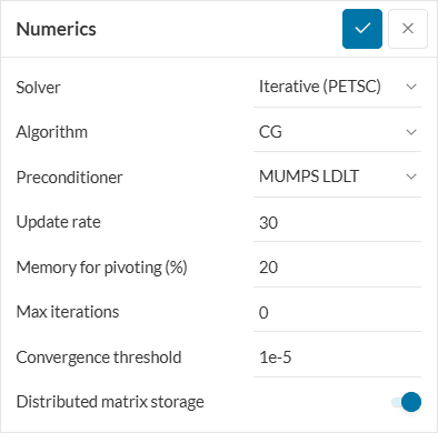
- Algorithm: Selects the solution algorithm.
- CG: Conjugate Gradients
- CR: Conjugate Residuals
- GCR: Generalized Conjugate Residuals.
- GMRES: Minimal Generalized Residuals, is the best compromise between robustness and speed.
- Preconditioner: Additional to the two common algorithms, the following options are available for this solver:
- Jacobi: Diagonal preconditioning.
- SOR: Successive over-relaxation.
- Inactive: No preconditioning of the matrix is performed.
- Renumbering method: Algorithm for pre-processing of the matrix.
- RCMK: Reverse Cuthill-McKee
- Inactive
Chronos
Fast and robust iterative solver. It is available for the linear static and thermomechanical analysis types.
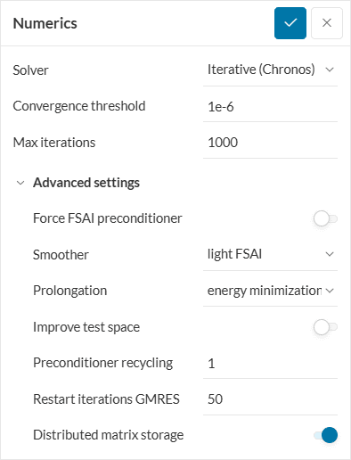
- Force FSAI preconditioner: Forces the usage of the FSAI preconditioner, can be faster for small problems.
- Smoother: Numerically challenging problems should use medium or heavy FSAI, which makes the solution more stable but also more expensive.
- Prolongation: Large problems should choose energy minimization, which makes the solution more stable but also more expensive
- Improve test space: Should be enabled especially for nonlinear or otherwise very challenging problems.
- Preconditioner recycling: Determines how often the preconditioner should be recomputed, thus has a significant impact on performance.
- Restart iterations GMRES: Specifies how often the search space is reset to improve computational efficiency and avoid excessive memory usage.
Nonlinear Equations Solver
A nonlinear equation solver is aimed towards finding the solution to a general non-linear equation of the form:
$$ F(x)=0 $$
Where \(x\) is a set of unknowns to be computed so that the equality is satisfied. In an FEA simulation, the nonlinear equation models the equilibrium of the structural system, and the searched solution is the set of deformations at each node (generally speaking, the degrees of freedom). Nonlinearities are introduced into the equations of equilibrium by conditions such as large deformations and rotations, nonlinear material deformations, and physical contacts.
Generally, an explicit analytical solution to the equilibrium equation is not known, thus a numerical ‘search’ process is carried out to approximate it. The search process for the solution at each loading step is based on the Newton-Raphson method, and for it two versions are available:
- The classical, vanilla method of Newton-Raphson, which iterates at each loading step over the deformations until the imbalance of the internal and external forces (called the residual), is minimized below a given tolerance.
- The method of Newton-Krylov, which works in tandem with an iterative linear solver, unifies the residuals in the linear solution and the load imbalance at each loading step, to avoid running additional iterations and thus saving on computation time.
The parameters of the nonlinear solvers in SimScale are as follows:
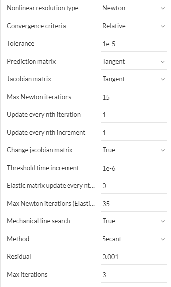
- Nonlinear resolution type: Select between the available variations of the Newton algorithm:
- Newton: Uses the classical, full ‘exact’ method for the resolution of the nonlinear system of equations at each loading step.
- Newton-Krylov: Uses an ‘approximate’ method of resolution, which leverages an iterative solution of the linear equations to save on computational time. (The Newton-Krylov variant is only available when using an iterative solver)
- Convergence criteria: Selects the definition of the residual used to evaluate convergence of the Newton iterations. The residual is defined as the difference between the internal and external forces, and can be optionally normalized to the magnitude of the external forces in the case of the Relative criteria. The default setting is to use the Adaptive criteria.
- Relative: The residual is computed by normalizing the imbalance between internal and external forces to the magnitude of the applied external forces.
- Absolute: The absolute imbalance is not normalized but compared directly to the tolerance value.
- Adaptive: A combination of both Relative and Absolute criteria is used. At each Newton iteration, the Relative criteria is used by default. In the case that the external loads vanish, the Absolute criteria is used instead.
- Tolerance: Threshold value for the residual. When the residual falls below this value, the iterations on the current loading step are considered to be converged.
- Prediction matrix: Select the stiffness matrix to be used at the first iteration in each loading step:
- Tangent matrix: Takes into account the non-linearities in the system for the calculation of the matrix.
- Elastic matrix: Only considers the elastic properties of the system for the calculation of the matrix (Young’s modulus and not the tangent modulus, given or deducted from the material law)
- Jacobian matrix: Select the stiffness matrix to be used in the iterations after the first one:
- Tangent matrix: Same as above.
- Elastic matrix: Same as above.
- Max Newton iterations: Allowable number of iterations to be carried at each loading step. After these iterations are performed, without the convergence criteria being met, the solution is considered to have diverged. If automatic time stepping is being used, the time step will be cut. Also, the solver is allowed to run additional iterations if the residual is expected to reach the threshold value, according to the Additional percentage of newton iterations (see Simulation control).
- Update every nth iteration: After this many number of iterations, the acobian matrix will be recomputed. If set to zero, the matrix is not updated inside each loading step.
- Update every nth increment: After this many number of loading steps, the jacobian matrix will be recomputed. If set to zero, the matrix is not updated in the whole process.
- Change jacobian matrix: Select if the jacobian matrix will be changed from tangent to elastic matrix if the time step falls below the given threshold in a load discharge process. This condition is valid under the consideration that the non-linearities do not evolve after small time increments.
- Threshold time increment: If the time increment falls below this value, the jacobian will use the elastic matrix for load discharge.
- Elastic matrix update every nth iteration: Frequency of updating of the elastic matrix under load discharge.
- Max Newton iterations (Elastic Jacobian): Override of the maximum number of allowable iterations, taking into account the fact that convergence is slower when using the elastic matrix.
- Mechanical Linear Search: Used to help the convergence of the Newton method, specially when not using the jacobian tangent matrix. When the jacobian matrix is too ‘soft’ (for example, plasticity zones allowing large deformations), the Newton approximation can fall far away from the current point. Linear search limits this divergence, with a criteria based on the ‘softness’ of the tangent matrix.
- Method: Selects the algorithm of line search, between:
- Secant: Unidimensional secant method.
- Mixed: Secant method with variable bounds.
- Residual: Threshold value for the residual in the linear search to be considered converged.
- Method: Selects the algorithm of line search, between:
Max iterations: Maximum allowed number of iterations in the linear search.
Time Integration
Time integration appears in transient models, in which the inertial effects are taken into account. Such models are often referred to as ‘Dynamic’, because they can be described by general the second-order dynamics equation:
$$ M\ddot{u}+C\dot{u}+Ku=L(t) $$
The task of a numerical integration algorithm is to compute the displacement, velocity and acceleration fields at a finite number of time steps. This algorithm works in conjunction with a non-linear equations solver to take into account big displacements, material nonlinearities and physical contact.
Four time integration algorithms are available, grouped into two broad categories: implicit and explicit time schemes:
- Implicit integration
- Newmark
- Hilber-Huhges-Taylor (HHT)
- Explicit integration
- Central differences
- Tchamwa time integration scheme
The available parameters to control time integration are:
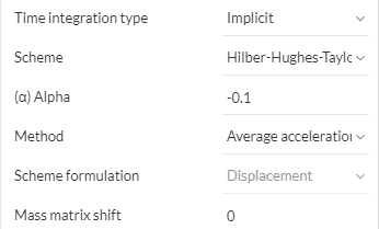
- Time integration type: Selects between an implicit or explicit integration schemes:
- Implicit: The field at the next time step is computed using information of its future first and second derivatives. This makes it possible to use larger time steps, at the expense of higher computational cost.
- Explicit: The field at the next time step is computed using information exclusive of the derivatives at the current time step. This causes a lower computational cost at each step, but an upper limit on the time step size. These schemes are preferred in problems of fast-dynamics, that is, involving pressure-wave propagation.
- Scheme: For each time integration type, a specific algorithm is selected, and its corresponding parameters are specified:
- (Implicit) Newmark: The numerical parameters control the accuracy and numerical damping in the integration (that is, the artificial energy loss due to approximation errors). For example, the trapezoidal rule with no numerical damping is achieved with values of \(\beta\) = 1/4 and \(\gamma\) = 1/2.
- \((\beta)\) Beta: Numerical parameter of the scheme
- \((\gamma)\) Gamma: Numerical parameter of the scheme
- (Implicit) Herber-Hughes-Taylor: a variation of the Newmar scheme, relates the \(\beta\) and \(\gamma\) parameters to a unique \(\alpha\) parameter.
- \((\alpha)\) Alpha: numerical parameter of the scheme. Must be negative or zero to guarantee that the integration is unconditionally stable.
- Method: The methods change the numerical damping of the scheme, in terms of the damping being proportional or inversely proportional to the frequency of the phenomena, given the same value of \(\alpha\):
- Alpha method: Lower frequencies are more damped than higher frequencies.
- Modified Acceleration: Higher frequencies are more damped than lower frequencies.
- (Explicit) Central differences: Based in the method of newmark, but does not induce any numerical damping.
- (Explicit) Tchamwa-Wielgosz time integration scheme: Introduces some numerical damping at higher frequencies.
- \((\varphi)\) Phi: numerical parameter for the scheme, controlling the amount of damping at higher frequencies.
- (Implicit) Newmark: The numerical parameters control the accuracy and numerical damping in the integration (that is, the artificial energy loss due to approximation errors). For example, the trapezoidal rule with no numerical damping is achieved with values of \(\beta\) = 1/4 and \(\gamma\) = 1/2.
- Stop on CFL criterion: For explicit schemes, stop the computation if the time step is smaller than the threshold value given by the Courant-Fredrichs-Lewy criteria.
Mass matrix shift: It is possible to add the scaled stiffness matrix to the mass matrix to improve the convergence in implicit schemes. The scaling factor of the added stiffness matrix is the given coefficient.
Modal Solvers
Modal analysis is used to study the natural vibration or buckling modes of a structure. The task of the modal solver is to find the solutions to the eigenvalue equation (general or quadratic), which requires to find the values:
$$ (\lambda, u) $$
Such that:
$$ (A – \lambda B) u = 0 \tag{GEP} $$
$$ (A + \lambda B + \lambda^2 C) u = 0 \tag{QEP} $$
Where the vector \(u\) is the vector of degrees of freedom and the coefficient matrices \( A, B, C \) are derived from the structural mass, damping, stiffness and gyroscopic matrices.
There are four modal solvers available, all of them using the subspace technique, which means that they approximate the solution by reducing the size of the numerical problem. The exception to this is the QZ method, which performs an exhaustive search for the modes, and thus gives the solutions of reference. The following table compares the methods:
| Solver | Application | Benefits | Disadvantages |
|---|---|---|---|
| IRAM – Sorensen | Compute a portion of the modes | Robustness. Best resource management. Quality control of the modes Treats asymmetric real matrices | Not asymmetric + complex matrices |
| Lanczos | Compute a portion of the modes | Detection of rigid body modes | Only real symmetric matrices |
| Bathe – Wilson | Compute a portion of the modes | Not very robust. Only real and symmetric matrices | |
| QZ | Compute the totality of modes | Most robust Reference method | Resource intensive Only useful for problems with less than 1e4 degrees of freedom |
The available parameters for each solver are:
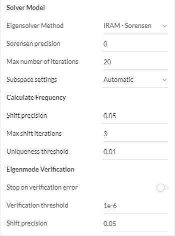
IRAM – Sorensen
- Sorensen precision: Numerical convergence threshold for the modes. The default zero value uses machine precision (~10^-16).
- Max number of iterations: Authorized number of restarts of the Sorensen method.
Lanczos
- Orthogonality precision: Numerical convergence threshold for the orthogonalization of the modes.
- Max orthogonality iterations: For the numerical orthogonalization of the modes.
- Lanczos precision: Criteria to determine the nullity of a term in the computation of the reduced problem.
- Max QR iterations: For the solution of the reduced system with the QR method.
- Rigid body modes detection: Compute preliminary the rigid body modes. If the rigid body modes are computed with this option off, the eigenvalues will not be exactly zero but close to zero.
Bathe – Wilson
- Bathe precision: Numerical convergence threshold for the modes in the Bathe & Wilson method.
- Max Bathe iterations: Authorized number of iterations for the Bathe & Wilson method.
- Jacobi precision: Numerical convergence threshold for the modes in the Jacobi method.
- Max Jacobi iterations: Authorized number of iterations for the Jacobi method.
Subspace settings
Common to the three solvers above. Allows overriding the automatic computation of the subspace size used to efficiently find the modes.
- Automatic: The solver determines the size of the subspace.
- Dimension: Directly specify the size of the subspace.
- Coefficient: The dimension of the subspace is this value times the number of searched modes.
QZ
- Type: Allows to select the variants of the algorithm between Simple, Equi and QR.
Other general settings are available for the modal solution, named the frequency calculation (‘Calculate Frequency’) and the mode postprocessing (‘Eigenmode Verification’):
Calculate Frequency
- Shift precision: Allow to extend the search range (upper or lower) limit or “shift it” by this amount when an eigenvalue is found to be close to the limit.
- Max shift iterations: Number of times that the algorithm can shift the limit of the search range.
- Uniqueness threshold: Threshold to determine that an eigenvalue is considered to be zero.
Eigenmode Verification
- Stop on verification error: Allow the solver to exit the computation if the numerical threshold or the Sturm test criteria are not met.
- Verification threshold: Tolerance for the convergence residual that determines if a mode is incorrectly computed, and a verification error should be raised.
- Shift precision: Percentage used to define the interval (with respect to an eigenvalue) on which the Sturm test will be carried.
The Sturm test is used to verify that the algorithm has found the exact number of eigenvalues in the requested range.
References
- Code Aster U2.08.03 – Note of use of the linear solvers.
- Code Aster U4.50.01 – Keyword SOLVEUR.
- Code Aster U4.51.03 – Operator STAT_NON_LINE.
- Code Aster R5.03.01 – Quasi-static nonlinear algorithm.
- Code Aster R5.05.05 – Dynamic nonlinear algorithm.
- Code Aster R5.01.01 – Modal solvers and solving generalized eigenvalue problems (GEP).
- Code Aster U4.52.02 – Operator CALC_MODES.
Last updated: March 13th, 2025
Did this article solve your issue?
How can we do better?
We appreciate and value your feedback.


