Mesh Quality

This standard documentation covers what is mesh quality and why it’s important. Before starting to read this document, we strongly recommend checking out the following articles:

As mentioned in the mesh article, a mesh is the discretization of geometry into individual elements. Since the mesh is an approximation of the actual geometry, the mesh density and quality have a significant influence on the accuracy and stability of a simulation.

The purpose of mesh quality metrics is to assess the suitability of a discrete computational domain (Mesh) for simulations. A mesh is usually considered to be of higher quality compared to another mesh if it improves at least one of the most important simulation properties; Time to convergence, stability or accuracy without affecting the others negatively.

1. Mesh Quality Metrics

We measure the mesh quality, using a set of quality metrics. The quality metrics determine how far we are from an ideal cell shape. Below, you will see some mesh quality metrics used in SimScale.

1.1 Aspect Ratio

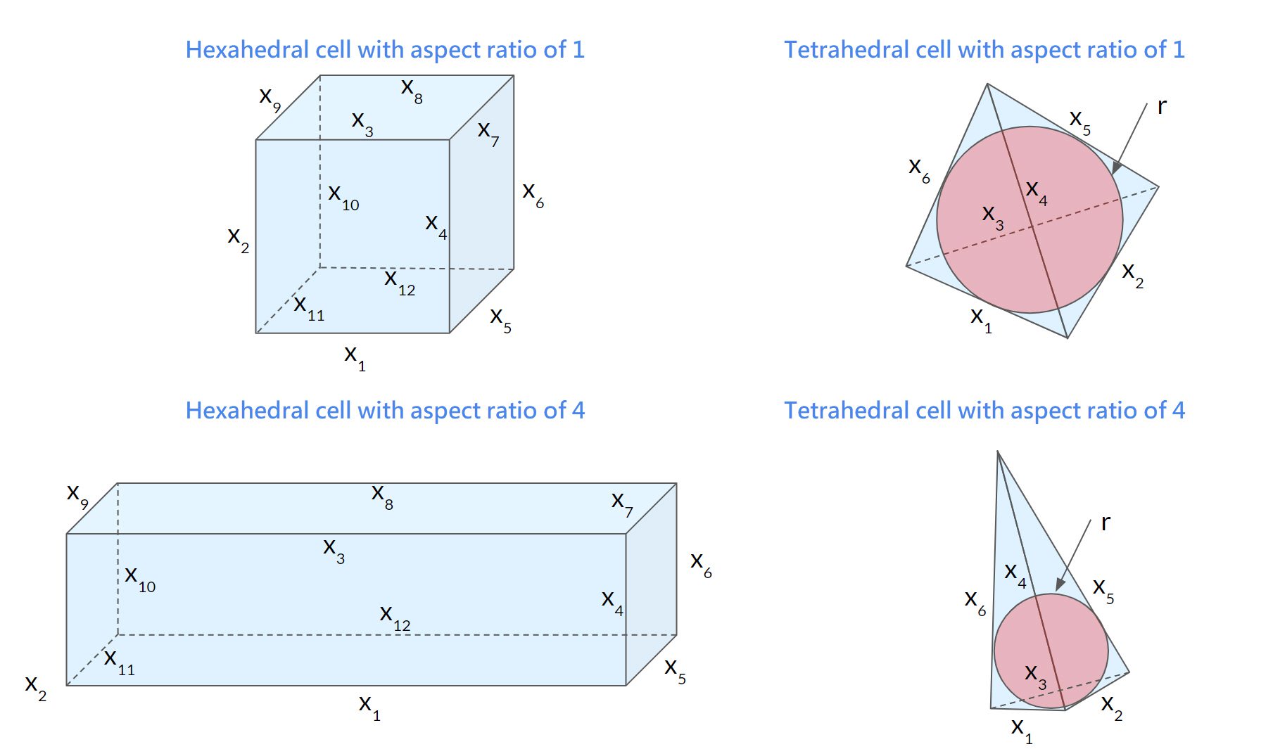
Briefly, the aspect ratio is the ratio of a cell’s longest length to the shortest length. The ideal aspect ratio is 1. The smaller it is, the higher the quality of an element is. The calculation method varies by the cell type as follows:

Hexahedral cell aspect ratio: Ratio of maximum edge length to the minimum edge length.

$$ AspectRatio = \frac{max(x_1, x_2, …, x_{12})}{min(x_1, x_2, …, x_{12})} $$

Tetrahedral cell aspect ratio: It’s correlated between the maximum edge length and radius of the cell’s internal sphere.

$$ AspectRatio = \frac{max(x_1, x_2, …, x_6)}{2 \cdot \sqrt 6 \cdot r} $$

high and low aspect ratio of hexahedral and tetrahedral elements — Figure 1: Comparison of high and low aspect ratio per element type

1.2 Non-orthogonality

Non-orthogonality is the angle between the vector connecting two adjacent cell centers and the normal of the face shared by these cells. The range of non-orthogonality is between 0 (ideal) and 90 (worst). 0 indicates the mesh being orthogonal. Two perfect hexes aligned with each other have non-orthogonality equal to 0.

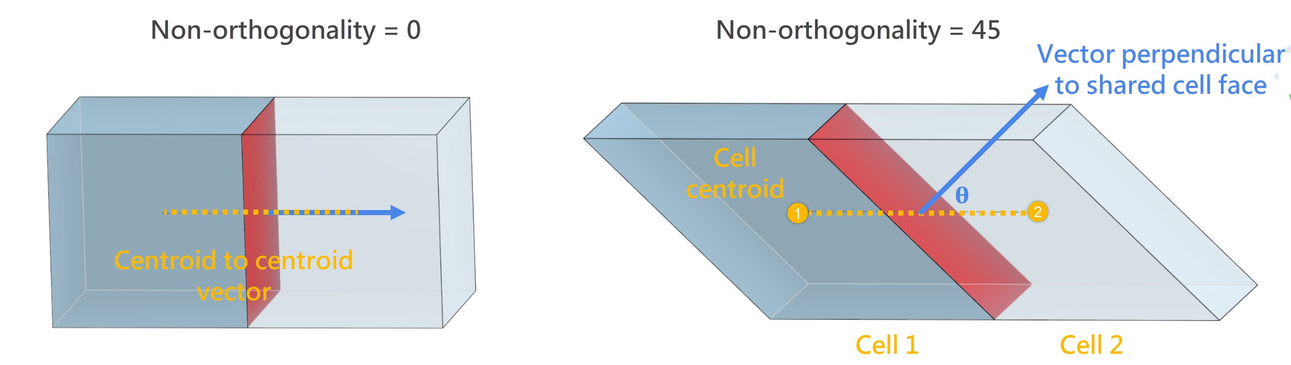
comparison of a low and high non-orthogonality on hexahedral cells — Figure 2: Representation of non-orthogonality mesh quality metric based on cell centroid and shared cell face

A high level of non-orthogonality should be avoided since it causes numerical instability. As a result, the simulations with higher non-orthogonality either take longer to converge, or even diverge.

It is recommended to keep the non-orthogonality below 70. Please consider improving the mesh if the non-orthogonality is above 80. Simulations with the meshes with maximum non-orthogonality above 85 likely diverge.

1.3 Volume Ratio

Volume ratio is the ratio of the volumes of the adjacent cells. Consider two adjacent cells with volumes of $V_1$ and $V_2$. The volume ratio is computed as follows:

$$ Volume\ ratio = \frac{max(V_1, V_2)}{min(V_1, V_2)} $$

In reality, a single cell is surrounded by multiple neighbor cells. Since there are multiple volume ratios, we consider the maximum volume ratio as the cell’s volume ratio.

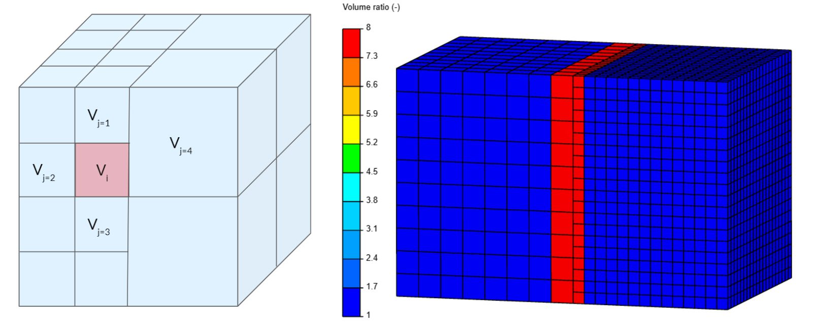
small and large hexahedral cells around a cell shows how the volumeratio mesh quality metric is calculated — Figure 3: Volume ratio is a mesh quality metric that is a function of the sizes of neighbor cells.

$$ Volume\ ratio_i = max( Volume\ ratio_{j=1}, Volume\ ratio_{j=2},…, Volume\ ratio_{j=n}) $$

The ideal volume ratio is 1. The smaller it is, the higher the quality of an element is.

1.4 Tet Edge Ratio

Tet edge ratio is the ratio between the longest and the shortest edges. This quality metric is only available for the tetrahedral cells. Considering the edge lengths of a cell represented by x, the tet edge ratio is then computed as follows:

$$ Tet edge ratio = \frac{max(x_1, x_2, … x_6)}{min(x_1, x_2, … x_6) } $$

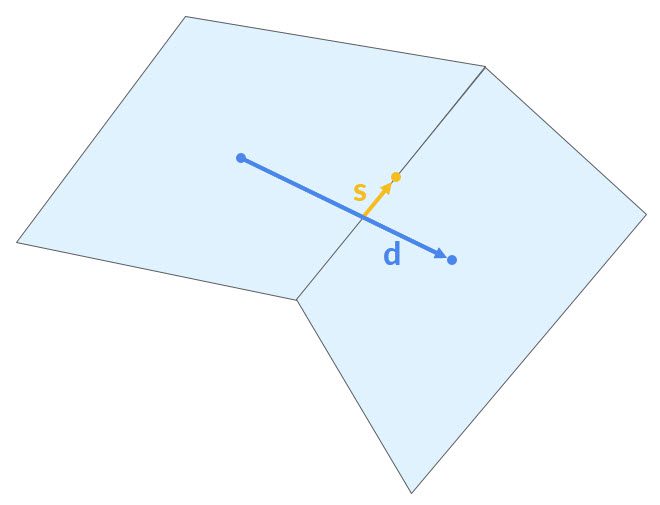
1.5 Skewness

Skewness is the normalized distance between a line that connects two adjacent cell centroids and the distance from that line to the shared face’s center. The range of skewness is between 0 (ideal) to $\infty$. Highly skewed cells are not preferred due to the poor accuracy they cause within the interpolated regions. The calculation method is as follows, for any cell type:

$$ Skewness = \frac{\mid \vec{s} \mid}{\mid \vec{d} \mid}$$

Where $\mid \vec{s} \mid$ is the norm of the skewness vector and $\mid \vec{d} \mid$ is the norm of the vector that connects the adjacent cell centroids, as shown in the Figure below.

Visual representation of skewness — Figure 4: Visual representation of the vectors that will be used to calculate Skewness.

1.6 QuadMaxAngle

Hexahedral cell quadMaxAngle is the maximum of the angles between neighboring cell edges. The normal range varies between 90 (ideal) to 180 (worst). The acceptable range is 90 to 135.

1.7 TriMaxAngle

Tetrahedral cell triMaxAngle is the maximum of the angles between neighboring cell edges. The normal range varies between 60 (ideal) to 180 (worst).

1.8 TriMinAngle

Tetrahedral cell triMinAngle is the minimum of the angles between neighboring cell edges. The normal range varies between 0 (ideal) to 60 (worst).

2. Quality Assessment

There are mainly two applications for this type of quality assessment:

Prior to running the simulation:
This is to ensure the mesh is a good fit for the upcoming simulation run. Evaluating at this level is more for CFD-experts, less experienced users can usually rely on the default settings.
After facing an issue in simulation:
If your solution diverges and the simulation fails, quality assessment gives you powerful tools at hand to identify problematic areas that can be, for example, fixed by adjusting the CAD model or refining certain areas in the mesh.

The following picture gives a preview of what the result of checking the mesh quality could look like:

visualisation of aspect ratio in a mesh for cfd analysis — Figure 5: Mesh metric aspect ratio for an example CAD model

2.1 Meshing Log

The quality of a mesh can be assessed by different metrics that are usually based upon the geometrical properties of the mesh cells (e.g. Aspect ratio) or upon the relation between neighboring cells (e.g. non-orthogonality). As the suitability of a mesh for a simulation is also strongly influenced by the simulated physics, the simulation solver, and the geometrical domain, the quality metrics can only give an indication if a mesh is a good fit for a simulation setup. As an example, you can find that simple incompressible CFD simulations are usually much less sensitive towards poor quality cells than compressible flow with high-density changes.

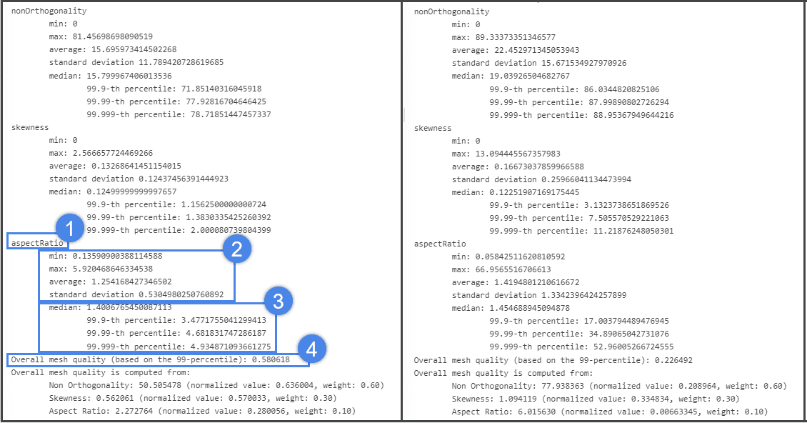
Figure 6 shows the meshing logs of a good and bad quality mesh. The marked points indicate:

Mesh quality metric
Minimum, maximum, average, and standard deviation of the corresponding quality metric within the mesh.
Median of the corresponding quality metric. Ensure that 99.9-th percentile of the metric is within the recommended range.
Overall mesh quality metric. Higher values indicate higher mesh quality.

visualization of meshing log in the simscale platform — Figure 6: Comparison of meshing logs of good (left) and bad (right) mesh qualities.

Best Practices for Mesh Quality Metrics:

The following table shows the maximum value for some of the meshing parameters beyond which the simulation is very likely to diverge. Low-quality meshes will most likely cause numerical errors and either fail the simulations or cause unreliable results. Note that some of the parameters are more/less relevant depending on the type of analysis to be performed (CFD/FEA).

Mesh Quality Metric	Maximum, CFD	Maximum, FEA
aspectRatio	—	30
TetAspectRatio	—	16
nonOrthogonality	88	—
skewness	—	10

Table 1: Maximum mesh quality metrics for CFD and FEA analysis types

Note

Volume ratio and non-orthogonality are defined on each face of the mesh. SimScale displays the maximum value for all faces which belong to a cell.

In the following examples, you will see the influence of low-quality mesh and high-quality mesh on simulation stability.

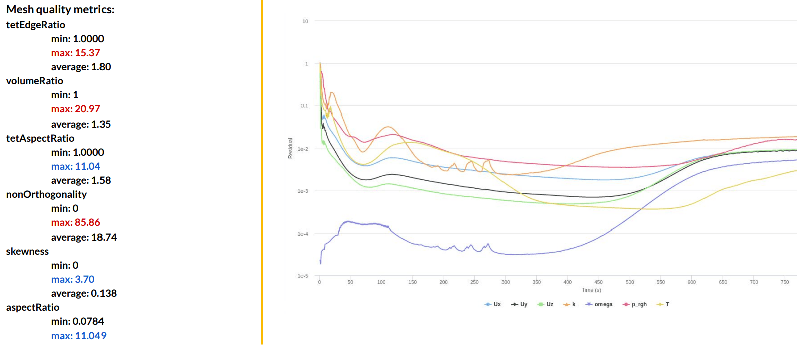
meshing log shows low mesh quality and convergence plot shows a diverged simulation — Figure 7: Example for a diverged simulation with a low mesh quality

The picture above presents the meshing log and convergence plot of a simulation with low-quality mesh. Low-quality mesh metrics are marked with red color. The convergence plot indicates that simulation diverged approximately after 400 iterations. The results from this simulation will be unreliable. For more information about convergence, please check the How to Check Convergence of a CFD Simulation? article.

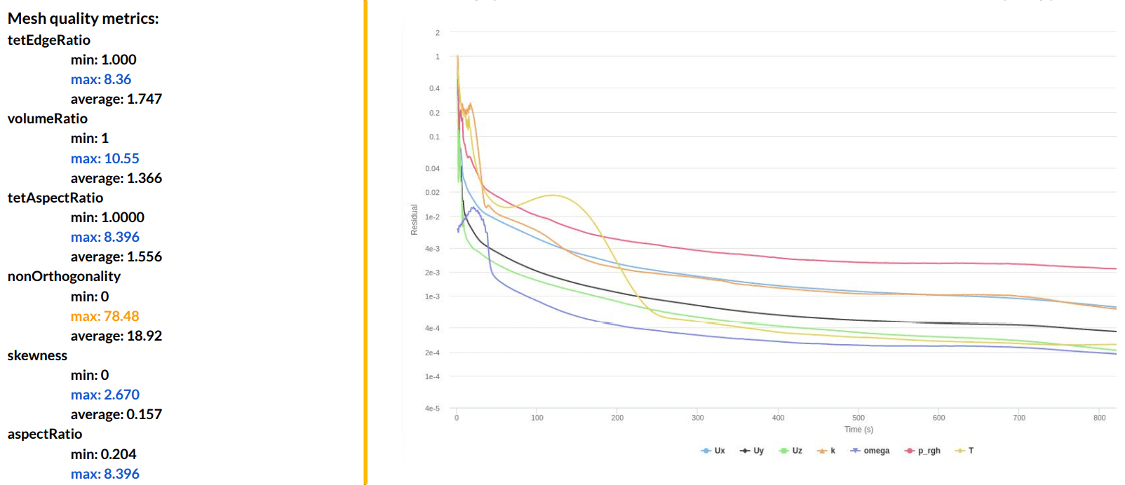
meshing log shows high mesh quality and convergence plot shows a successful simulation — Figure 8: Example for a successful simulation with a high mesh quality

Above, you see the meshing log and convergence plot from a successful simulation. High-quality mesh metrics are marked with blue color. The residual plot shows that the simulation is stable. This example shows that improving the mesh quality metrics created a significant impact on the simulation stability.

2.2 Mesh Visualization

Mesh quality metrics can be accessed in the navigation tree under ‘Mesh’ after the meshing is finished.

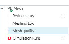
simscale simulation tree part for mesh visualization — Figure 9: Finding mesh quality in the simulation tree

The post-processing viewer loads the mesh and computes the mesh quality on the fly. It might, therefore, take up to a few minutes for big meshes (> 10 Million cells). You can display the different mesh quality metrics the same way result fields are displayed for simulation results.

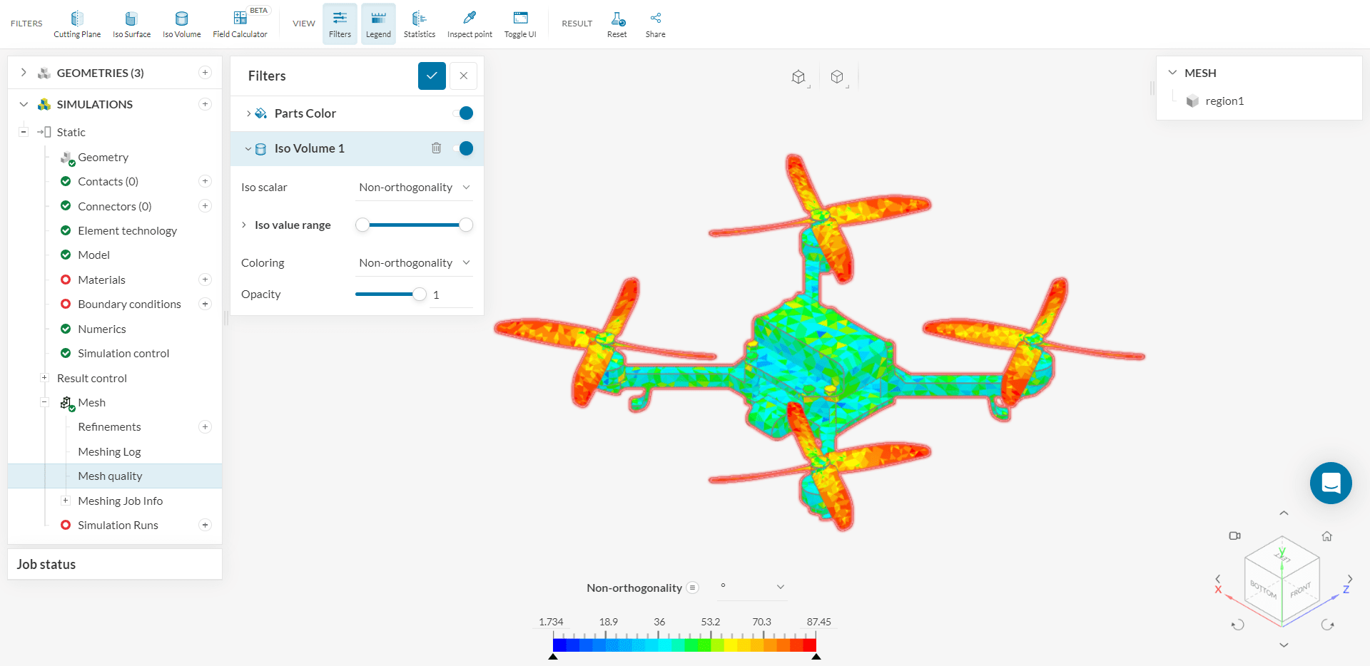
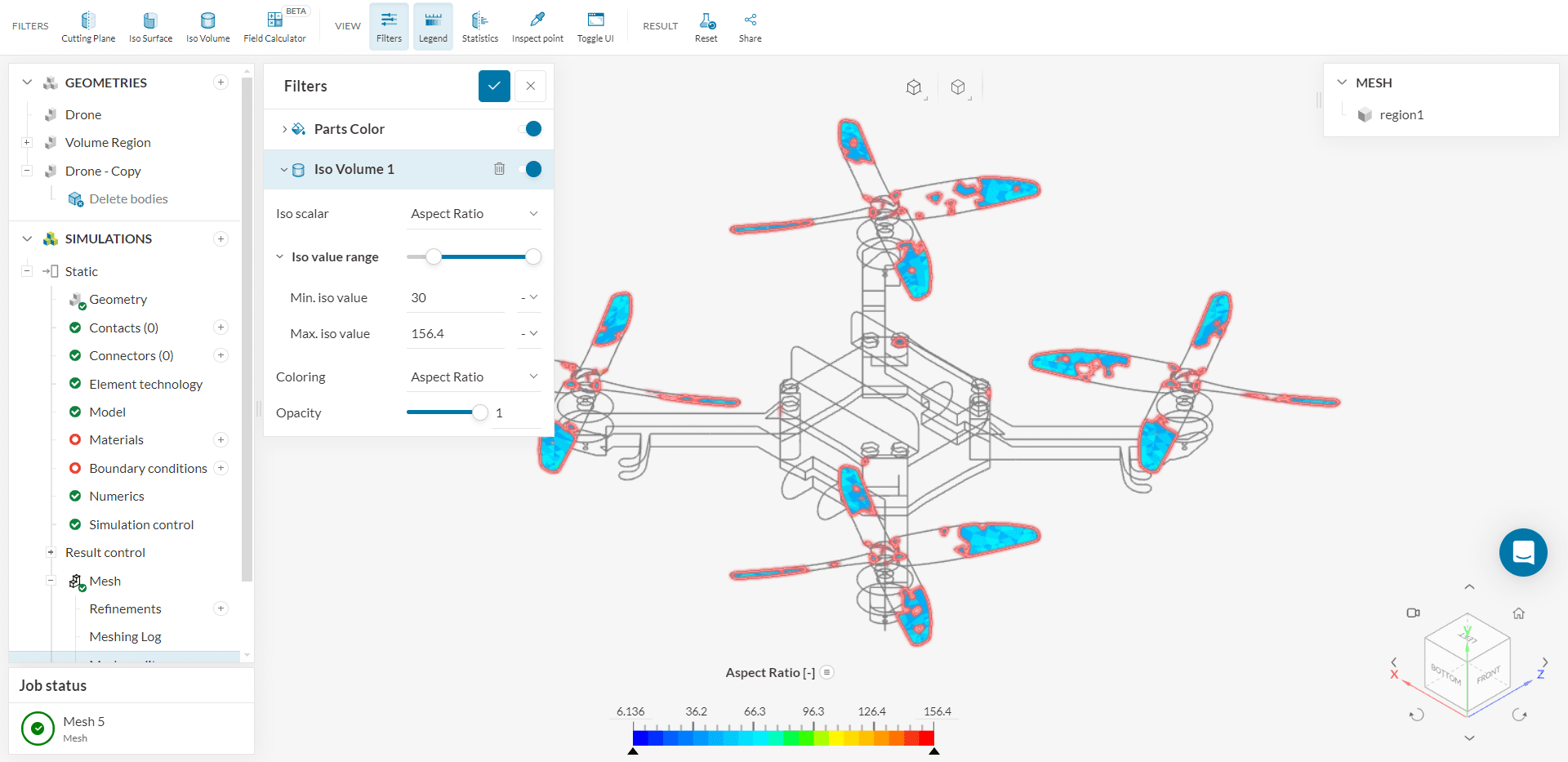
global distribution of non orthogonality degrees — Figure 10: Displaying a value over the surface of the whole domain.

2.3 Isolate Cells Based on a Metric

While all display filters are available for mesh fields, the Isovolume filter is especially handy. This filter allows you to isolate bad quality cells by adjusting the minimum or maximum threshold value to the recommended limits. The following picture shows how to create an Isovolume:

demonstration about how to create a insovolume to isolate the elements based on a limit and a metric to be shown — Figure 11: Isolating bad elements using *Isovolumes*

Open the Mesh quality feature.
Create a new Isovolume by clicking the ‘+’ button next to it.
Select the metric you want to analyze.
Use the sliders to adjust the limits of what you want to be displayed.

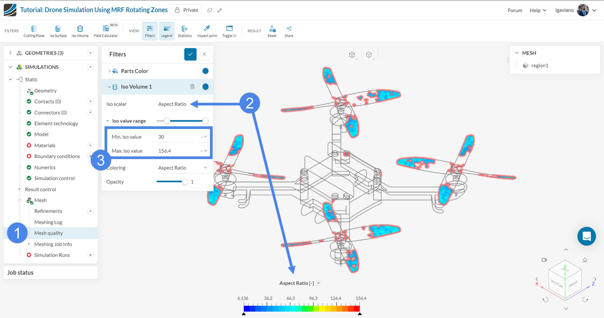
Sometimes the worst elements in the mesh will be very small, and when you try to isolate them, they will be hard or near enough impossible to spot. In such a case, it is helpful to hide the Parts completely and use the home button next to the orientation cube to zoom into the current extents of the visualization. In case there are tiny bad elements in several parts of the model, you may find yourself needing to restrict the Isovolume thresholds further. Once you have zoomed into the bad elements, you can then enable the Part visualization again to locate the cells within the model.

demonstration about how to utilize the home button for finding tiny elements in a mesh — Figure 12: Finding single elements in the whole domain by using the home button.

If you are wondering how to create good meshes, check out the meshing tutorial for the standard mesher.

3. Things to Do When the Mesh Quality is Low

Low mesh quality most likely causes numerical errors and cause divergence (simulation failure). In some cases, simulations do not fail but end up with unreliable results. Therefore, if you observe any of those problems, check the meshing log first. Compare the quality metrics with our best practices. If the metrics show that the mesh quality is insufficient, visualize the mesh, using the mesh quality tool. A complete mesh quality check and how to improve a mesh guide can be found in the How to check and improve mesh quality? article. In this article, you will find some practical measures to improve the mesh quality. This includes updating the CAD model and adjusting the mesh settings.

Our OpenFOAM solvers allow adjusting of the numerics. If the mesh quality is questionable, as a last resort, you may also adjust the numerics to overcome the mesh quality-related numerical errors.

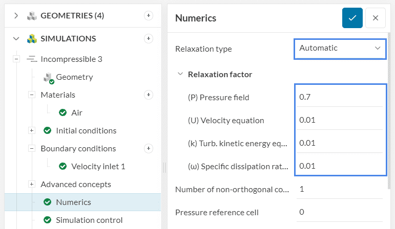
3.1 Relaxation Factors

You may adjust the relaxation factors to ‘Automatic’. For more information about the relaxation factors, check out the CFD Numerics: Relaxation factors page.

relaxation type and factors under simscale flow simulation numerics — Figure 13: Recommended automatic relaxation type

3.2 Non-orthogonal Correctors

Non-orthogonal correctors intend to correct the fluxes in the flow direction by repeating the pressure iterations. As a result, they increase the computational requirement. The increase in the Number of non-orthogonal correctors should be with respect to the maximum non-orthogonality metric:

If the max nonOrthogonality is below 75, no need for any non-orthogonal corrector.
If the max nonOrthogonality is between 75 and 82, use 1 non-orthogonal corrector.
If the max nonOrthogonality is between 82 and 85, use 2 non-orthogonal correctors.

If the max nonOrthogonality is above 85, better improve the mesh quality. In this case, it is no longer feasible to increase the number of non-orthogonal correctors.

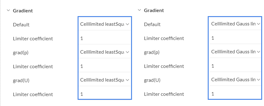
3.3 Gradient

The cellLimited scheme limits the gradient such that when cell values are extrapolated to faces using the calculated gradient, the face values do not fall outside the bounds of values in surrounding cells.

A limiting coefficient is specified after the underlying scheme for which 1 guarantees boundedness and 0 applies no limiting. Practically speaking, use 0 for accuracy and 1 for improving stability.

If the non-orthogonality is between 75 and 80, use cellLimited least squares 1.0.
If the non-orthogonality is above 80, use cellLimited Gauss linear 1.0.

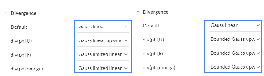
gradient settings under simscale flow simulation numerics — Figure 14: Recommended gradient settings for a high-quality mesh (left) and low-quality mesh(right)

3.4 Divergence

The divergence schemes are convective discretization schemes. Briefly, first-order schemes are easier to converge and second-order schemes are more accurate.

If the non-orthogonality is between 75 and 80, use second order schemes, such as Gauss linear upwind or Gauss limited linear.
If the non-orthogonality is above 80, use first order schemes, such as Bounded Gauss upwind.

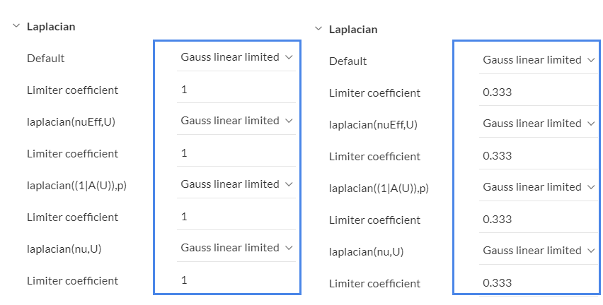
divergence settings under simscale flow simulation numerics — Figure 15: Recommended divergence settings for a high-quality mesh (left) and low-quality mesh(right)

3.5 Laplacian

Laplacian is a differential operator given by the divergence of the gradient of a scalar function. A typical Laplacian term is the diffusion term in the momentum equations. The limiter coefficient varies between 0 and 1.

Limiter coefficient 0: Uncorrected, bounded correction, 1st order, non-conservative. Suitable for low-quality meshes.
Limiter coefficient 1: Corrected, unbounded correction, 2nd order, conservative. Suitable for high-quality meshes.

You may use the following best practices in selecting the Laplacian schemes:

Non-orthogonality<70: Use Gauss linear corrected or Gauss linear limited corrected with Limiter coefficient 1.
75<Non-orthogonality<80: Use Gauss linear limited corrected with Limiter coefficient 0.5.
Non-orthogonality>80: Use Gauss linear uncorrected or Gauss linear limited corrected with Limiter coefficient 0.333.

laplacian settings under simscale flow simulation numerics — Figure 16: Recommended laplacian settings for a high-quality mesh (left) and low-quality mesh(right)

3.6 Surface Normal Gradient

Similarly to the Laplacian terms, use the following best practices for the Surface normal gradients:

Non-orthogonality<70: Use Gauss linear corrected or Gauss linear limited corrected with Limiter coefficient 1.
75<Non-orthogonality<80: Use Gauss linear limited corrected with Limiter coefficient 0.5.
Non-orthogonality>80: Use Gauss linear uncorrected or Gauss linear limited corrected with Limiter coefficient 0.333.