Documentation
The Multi-purpose analysis type offers an automated robust meshing strategy producing hexahedral cells suitable for the underlying solver, thereby reducing mesh generation times by huge margins. Because the mesh has a high quality, it requires fewer cells to achieve the same level of accuracy. It offers faster convergence at the cost of a reduced feature set. Some highlights of the mesher are:
Multi-purpose is a Finite Volume-based CFD solver with segregated pressure-velocity coupling using a proprietary variant of the SIMPLE\(^1\) algorithm. It provides the possibility to simulate both incompressible and compressible flow, either laminar or turbulent in a single framework. Turbulence is modeled using the RANS equations with the k-epsilon turbulence model for closure and proprietary wall functions for near wall treatment.
Multi-purpose supports steady-state as well as full transient analysis. In full transient analysis, the fluid flow is modeled in a time-accurate manner and any rotating component in the domain is solved using the sliding mesh approach.
Within SimScale, one can effortlessly set up a Multi-purpose simulation that involves the following steps:
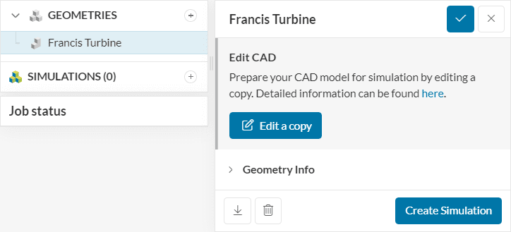
To create a Multi-purpose analysis, first, select the desired geometry and click on ‘Create Simulation’:
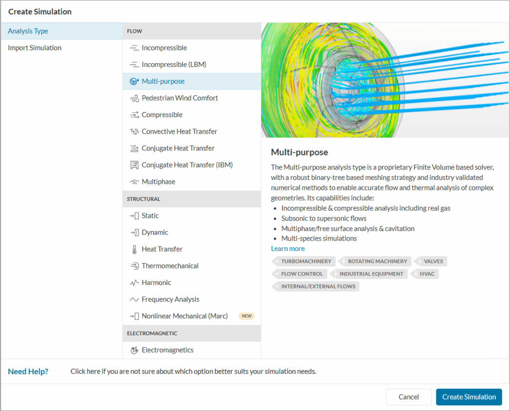
Next, a window with a list of several analysis types supported in SimScale will be displayed:
Important
Multi-purpose is a specialized analysis type restricted to users with a paid plan. For more details please visit our product & pricing page or contact sales.
Choose Multi-purpose analysis type and click on ‘Create Simulation’. This will lead to the SimScale Workbench with the following simulation tree and the respective settings:
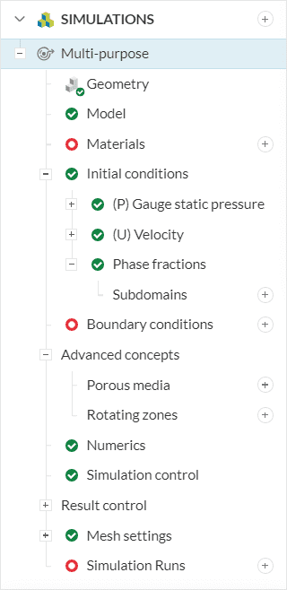
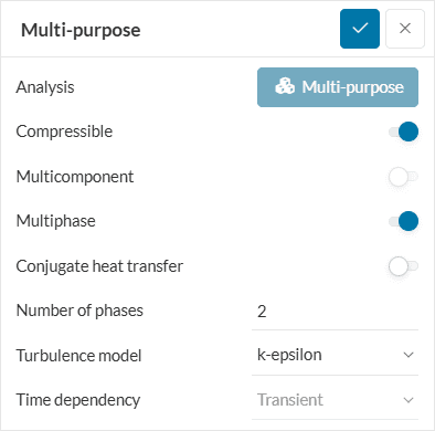
To access the global settings, click on ‘Multi-purpose’ in the simulation tree. The following parameters are available to define the fluid flow simulation:
The Geometry section allows you to view and select the CAD model required for the simulation. In general, having a clean CAD model always helps to avoid any meshing or simulation-related errors. However, the mesher is pretty robust and if the CAD is genuinely dirty then a message of mesh failure and further instructions on CAD cleaning or mesh refinement should appear.
Find more details about CAD preparation here.
If the simulation has a rotating component, then rotating zones need to be created for each rotating part. You can find a detailed approach to CAD preparation in the following article:
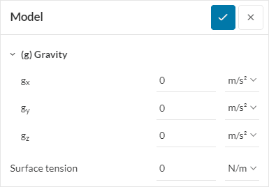
Under Model, gravity can be defined via a vector. The global coordinate system, represented by the orientation cube, applies to the direction of gravity. The vector coordinates \(g_x\), \(g_y\), and \(g_z\) represent the x, y, and z directions.
Surface tension can also be set for multiphase simulations. The default value of the surface tension coefficient is set to zero,
Under Materials, the appropriate fluid for the simulation can be chosen from the materials library. The user has the option to change certain fluid properties. For compressible simulations, since the temperature is involved the user needs to specify the corresponding thermophysical properties for the fluid in consideration.
Along with perfect gas behavior, it is also possible to model real gas behavior by specifying material properties as a function of pressure and temperature.
When Conjugate heat transfer toggle is enabled, it allows flexibility with the materials being used in the simulation. That is, users can choose the domain to consist of only flow regions, only solids, or a combination of both.
Real gas modelling
Fluids operating at very high pressure or low temperatures do not follow ideal gas behavior. For such ‘real’ fluids, more complex relations specifying the physical and thermodynamic properties are required, known as the real gas model.
For example, flow of refrigerant in compressors, flow of steam in a steam turbine, flow of gas mixture in a piping system etc.
To simulate real fluids the compressible flow toggle needs to be on under global settings as discused earlier.
For more information, please visit the relevant documentation page for materials.
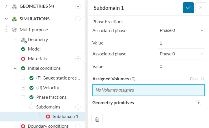
Initial conditions define the values which the solutions fields will be initialized with. For Multi-purpose analysis, Initial conditions can be set up in the simulation tree only when the multiphase is toggled on under global settings. The phase fraction can be initialized globally or for a specific region as a subdomain for all the phases involved.
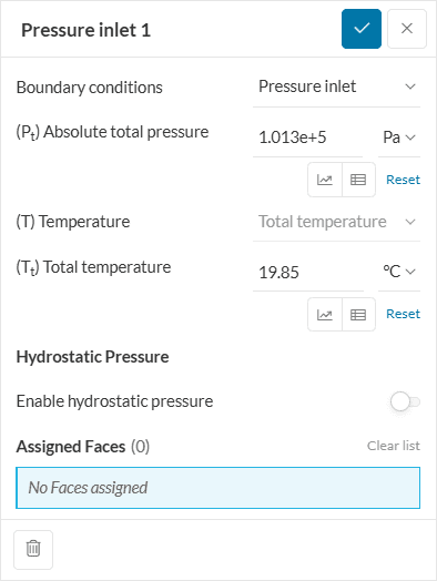
Boundary conditions help to add closure to the problem at hand by defining how a system interacts with the environment. In an incompressible simulation, the computational domain will be solved for two fields: pressure \((P)\), velocity \((U)\), while for a compressible simulation the temperature \((T)\) field is also involved. Additional turbulent transport quantities may be included based on the turbulence model selected.
The following boundary conditions are available for a Multi-purpose simulation:
Important
Parametric Studies
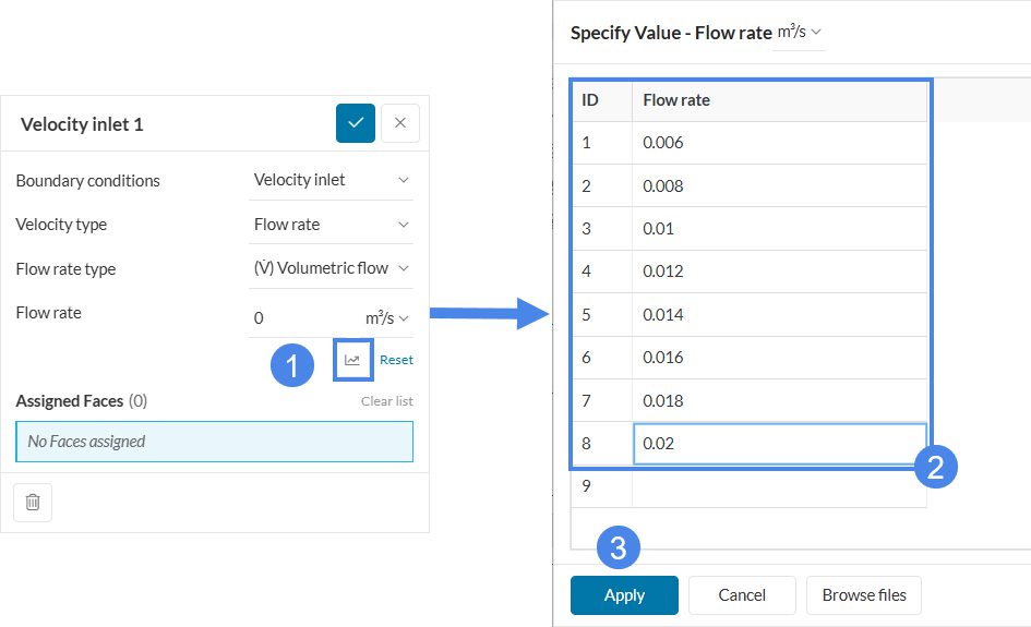
Multi-purpose analysis type allows parametric studies with the velocity boundary condition. When you select Flow rate as the velocity type while assigning velocity to an inlet or outlet face then you can input multiple flowrates at once either directly or by uploading a file.
This will initiate multiple runs with different flow rates assigned at once in parallel giving the user a huge time advantage.
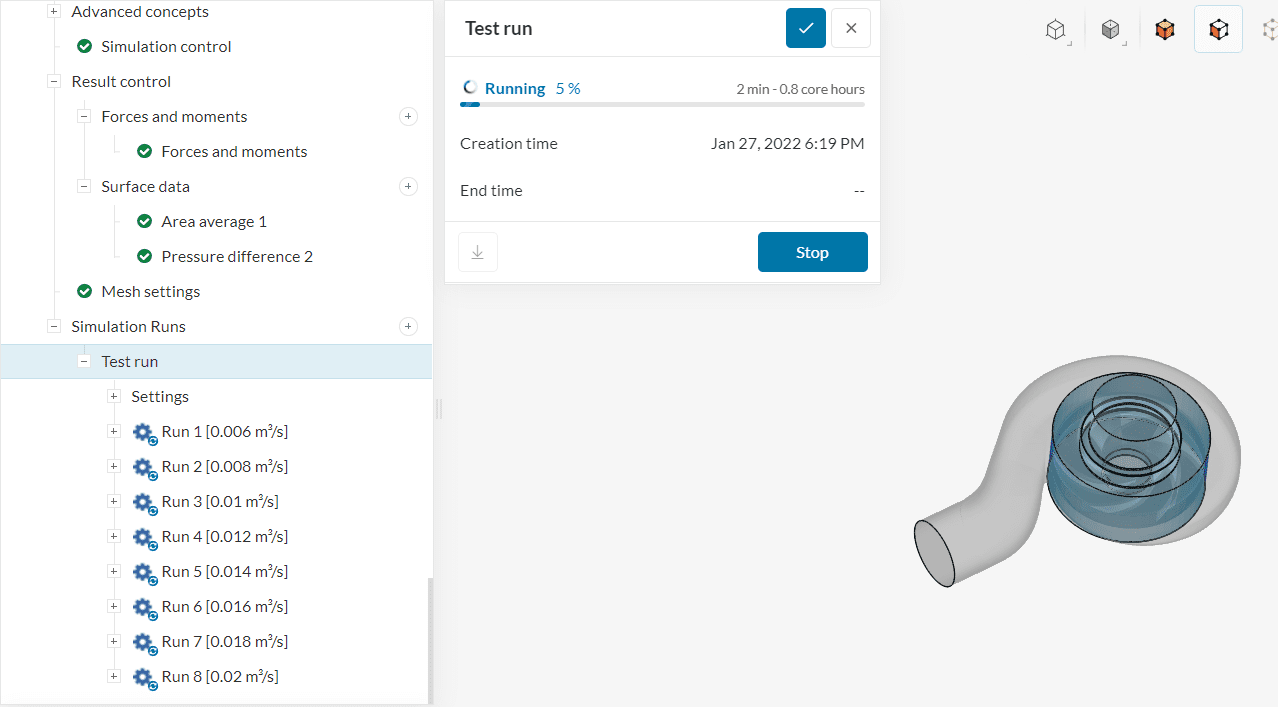
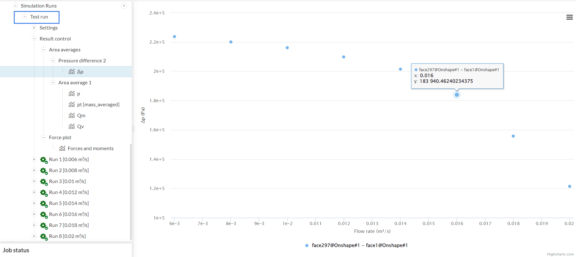
Results become available for individual flow rates as separate runs (Run 1, Run 2,……) and also for the complete parametric study where the whole parametric curve is plotted. Figure 11 shows the pressure difference curve for all 8 flow rates assigned under the simulation run named Test run by the user.
Under Advanced concepts, you will find additional setup options for rotating zones and porous media.
Numerical settings mainly influence the stability and efficiency of your simulation run, but also the quality of the results may depend on these settings. It is recommended to keep them at default settings.
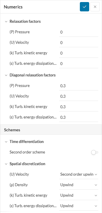
The difference between Numerics settings for Multi-purpose analysis and other OpenFOAM-based analyses is that in OpenFOAM-based we have a relaxation of the field and a relaxation of the equation – In Multi-purpose we have relaxation factors and diagonal relaxation factors for the fields.
The Simulation control settings define the general controls over the simulation. There are differences in the setup parameters, depending on the Time dependency of the analysis. Find below the differences between transient and steady-state analyses:
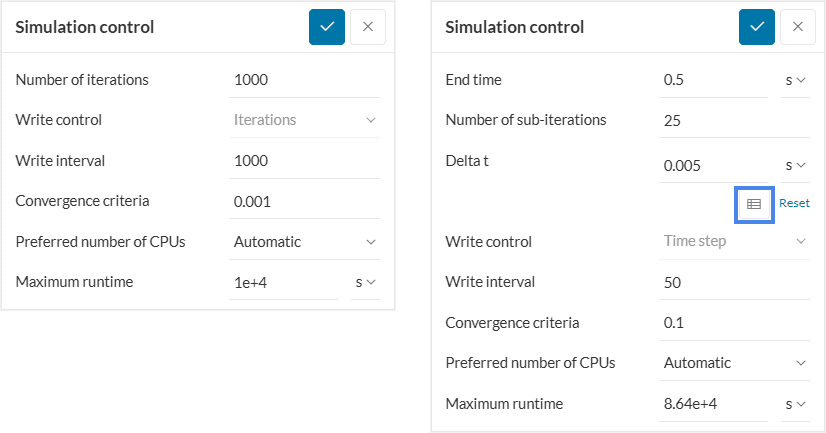
In the simulation control settings, there are only two parameters exclusive to the Multi-purpose analysis type:
For a complete overview of the other simulation control parameters and their meaning, please check out this page.
Figure 13 (right) highlights the table icon for defining Delta t. Manually defining a variable time step allows users to use a fine step at the start of a simulation and a coarser step later to reduce overall runtime and save core hours.
The Result Control section allows users to define additional simulation result outputs. It controls how the results will be written meaning the write frequency, location, statistics of the output data, etc. The following control items are supported:
For the Multi-purpose analysis type, the mesh generated is a Cartesian mesh which means that each cell represents a cube with edges parallel to the XYZ Cartesian axes making the mesh highly orthogonal.
The meshing algorithm is automated and follows a top-down approach which works by creating a binary tree structure. The bounding box (an imaginary box encompassing the dimensions of the flow domain) is refined anisotropically by cutting cells in the first layer (x-direction), in the second layer (y-direction), and the third layer (z-direction).
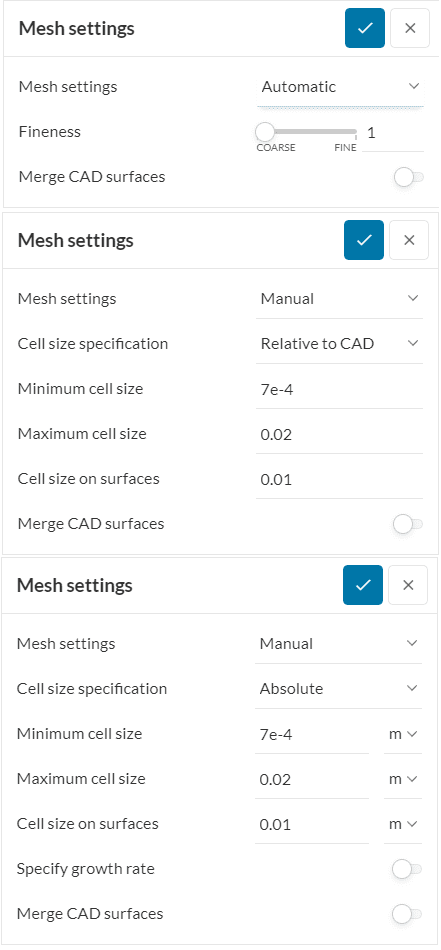
For the mesh in Multi-purpose analysis, the settings can be set to automatic or manual. The parameters under each mode are described below:
The user gets to define the following parameters:
The user gets to define the following parameters:
To apply additional mesh refinement to specific volume regions within the simulation domain, you can use a Region Refinement.
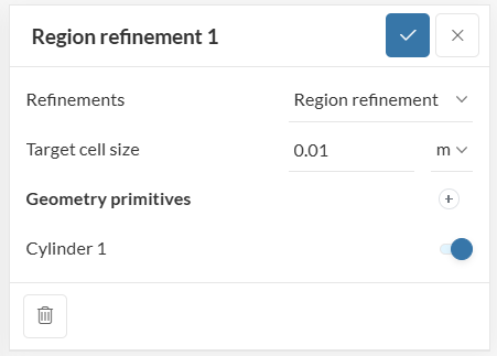
These volume regions or refinement zones can be created using geometry primitives.
Target cell size: This parameter specifies the length scale of all the Cartesian cells lying within the defined refinement zone. Note that the resulting cell size might be smaller than the target specified to accommodate the binary-tree mesh algorithm. Refer to the section Cell Size and Units for details on how the global meshing mode influences refinement units.
Smaller cell sizes mean larger mesh size and consequently longer simulation runtimes.
Note
The meshing log and the mesh are only visible once the simulation is finished. However, the time per iteration and the time to convergence are a lot lower compared to other solvers.
Your core hours will be consumed only after a successful
simulation run.
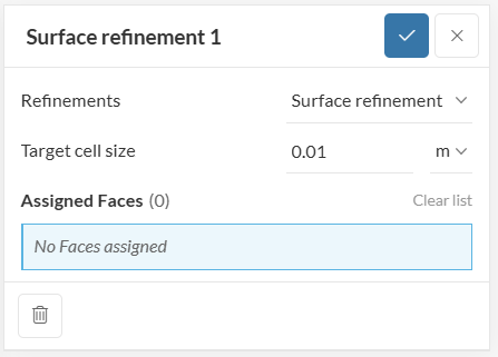
Surface refinements allow you to locally increase the mesh resolution on specific CAD surfaces without affecting the cell size in the rest of the domain. This gives you precise control over mesh quality in areas where geometry detail or flow physics demand it, while keeping the overall cell count manageable.
Typical scenarios where surface refinement is beneficial include:
Surface refinements are configured in the Mesh settings of a Multi-Purpose simulation. To add one:
Multiple surface refinements can be added, each targeting different surfaces with independent cell size settings.
The unit of the surface refinement Cell size depends on the meshing mode selected in the global mesh settings:
| Global mesh mode | Surface refinement unit |
|---|---|
| Automatic | Always absolute (meters) |
| Manual with absolute global cell size | Absolute (meters) |
| Manual with relative global cell size | Relative (fraction of the global cell size) |
Important
The surface refinement cell size must be smaller than the global cell size on surface. If the specified value is equal to or larger than the existing surface cell size, the refinement will be ignored and a warning will be shown before the mesh run starts.
Note
Surface refinement targets individual CAD faces and refines the mesh locally near those boundaries. It does not create a volumetric refinement zone. For refinement that extends into the volume of the domain, use a Region refinement instead.
Once all the settings are defined, click on ‘Simulation Runs’ to begin the simulation.
After the simulation is finished the SimScale’s integrated post-processor can be used to visualize the mesh as well as the simulation results.
As explained under Simulation control > Convergence criteria, convergence plots are available for post-processing during and after the simulation run. The following images show convergence plots for residuals for a steady-state and a transient simulation of an Ercoftac pump respectively.
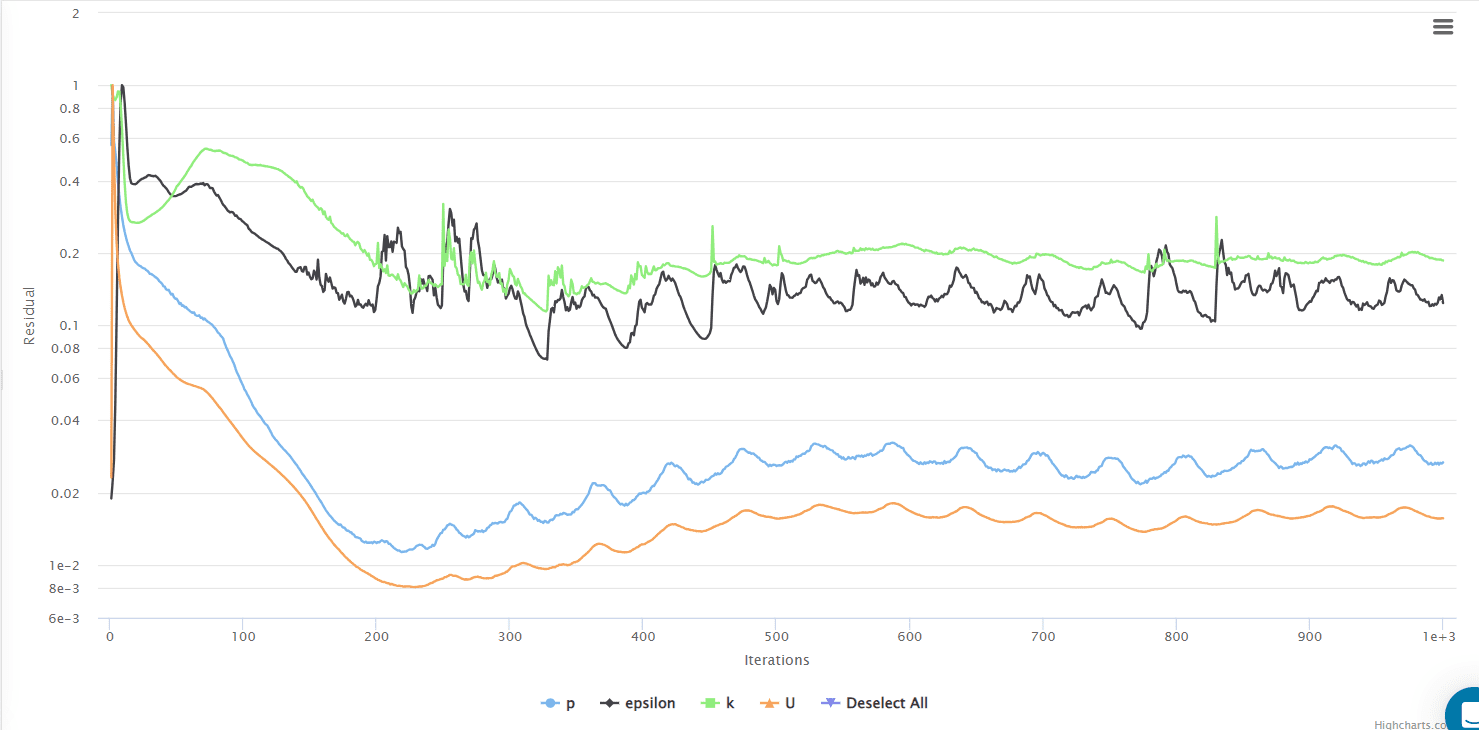
In Figure 17 the residual on the y-axis is a relative residual, the ratio between the residual at that iteration to the running maximum residual.
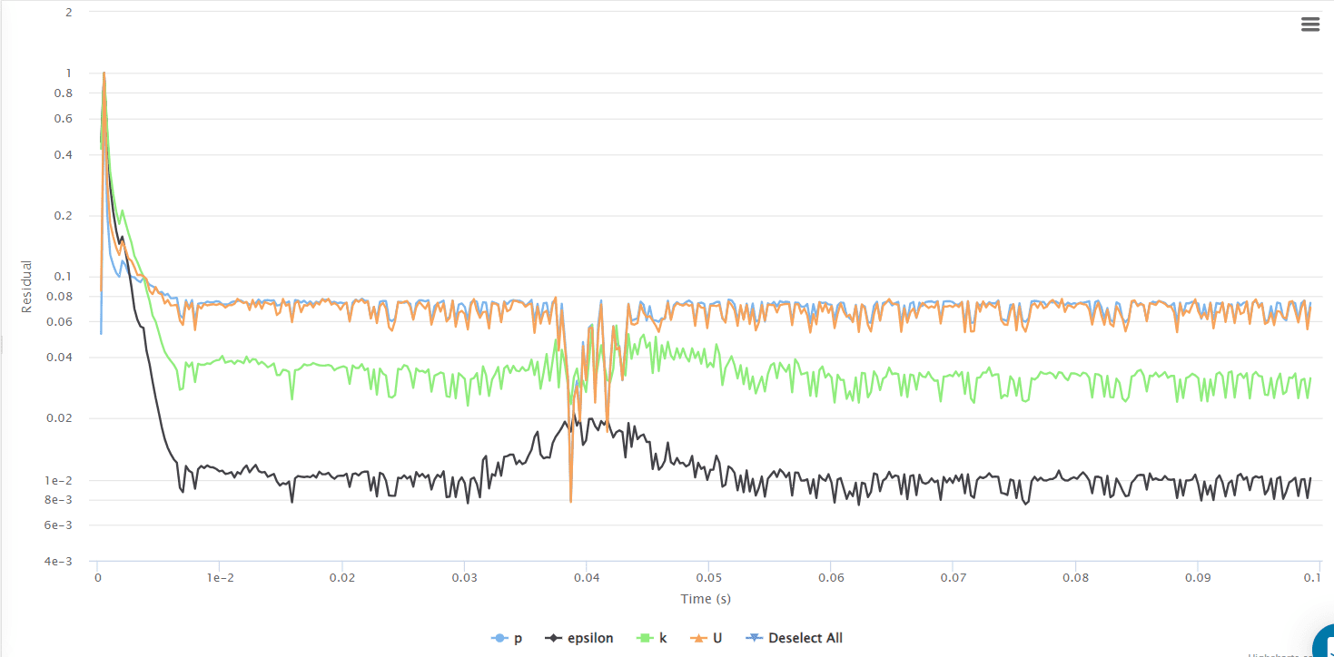
In Figure 18 the residual on the y-axis is a relative residual, the ratio between the residual at the last sub-iteration of that particular timestep to the running maximum residual.
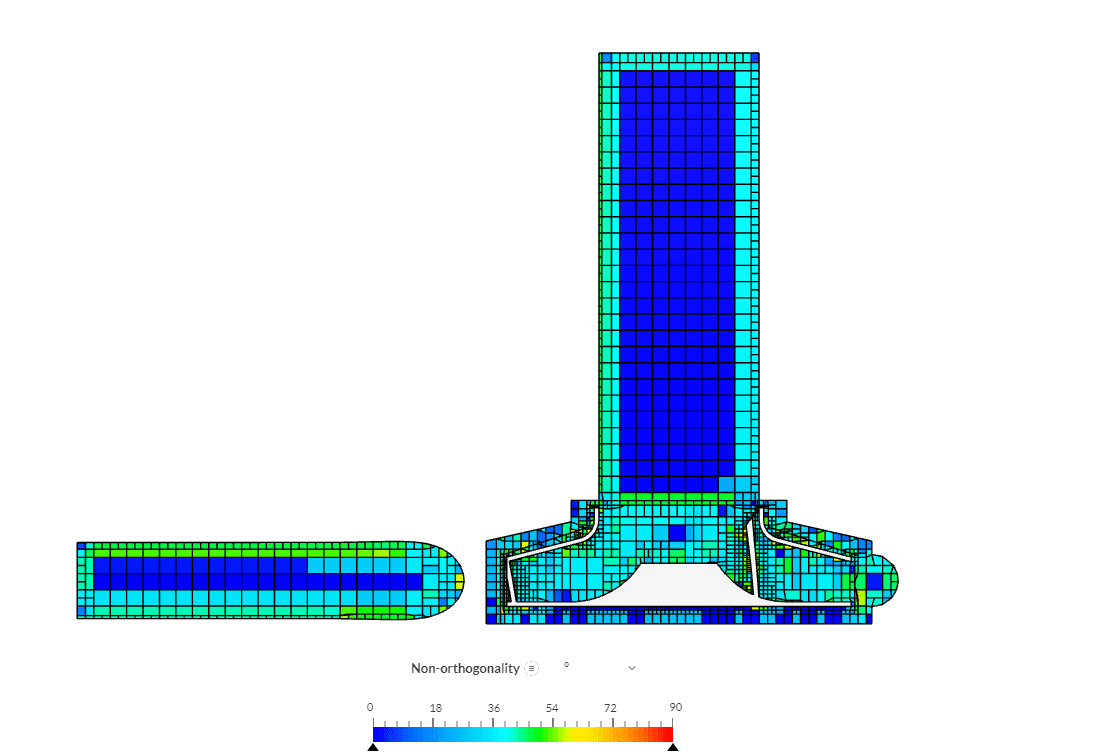
For a Multi-purpose simulation, the mesh quality parameters can be viewed within the SimScale’s integrated processor. This allows the user to inspect mesh criteria and use this information to improve the mesh. The following mesh parameters are available.
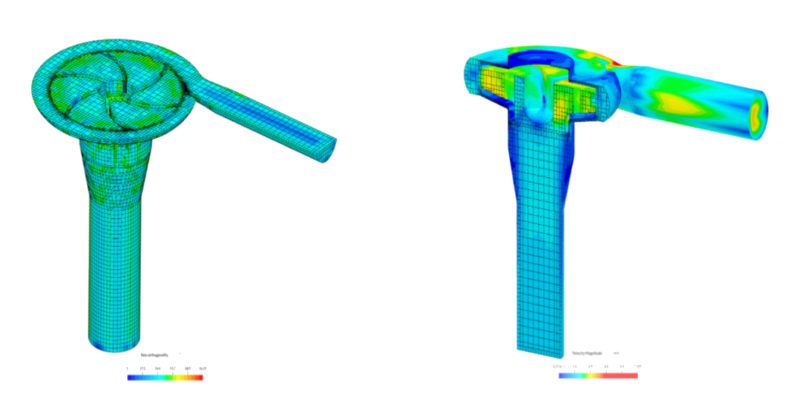
Mesh criteria can be displayed using various filters. Figure 19 shows an example of the non-orthogonality displayed on a cutting plane through a centrifugal pump. Please find more information on mesh quality parameters and the suggested mesh quality values here.
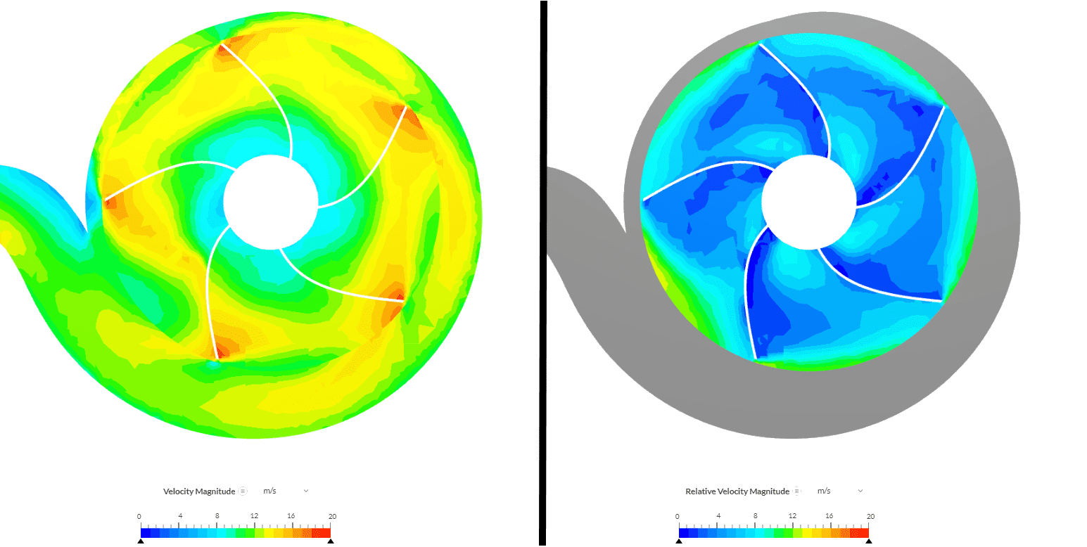
An additional Field Output only available in a Multi-purpose simulation is the Relative Velocity. This field function is used to evaluate the velocity of the fluid relative to the rotational velocity of the rotating region. It is applicable only within the rotating zone and every other region is greyed out. The relative velocity is calculated as in equation 1.
$$ Relative \ Velocity = Local\ Velocity\ – Rotational\ Speed \times Local\ Radius \tag{1} $$
The Local Velocity is the velocity at the centroid of a cell within the rotating zone and the Local Radius is the distance of the centroid of the cell to the origin of the rotating zone. By multiplying the Rotational Speed of the rotating region with the Local Radius the Local Rotational Velocity is calculated. Thus the Relative Velocity is calculated by subtracting the Local Rotational Velocity from the Local Velocity.
Figure 20 shows an example of the Local Velocity in comparison to the Relative Velocity.
Did you know?
An advantage of using Multi-purpose analysis involving rotating flows is that power about the axis of rotation is directly output.
Last updated: May 21st, 2026
We appreciate and value your feedback.
Sign up for SimScale
and start simulating now