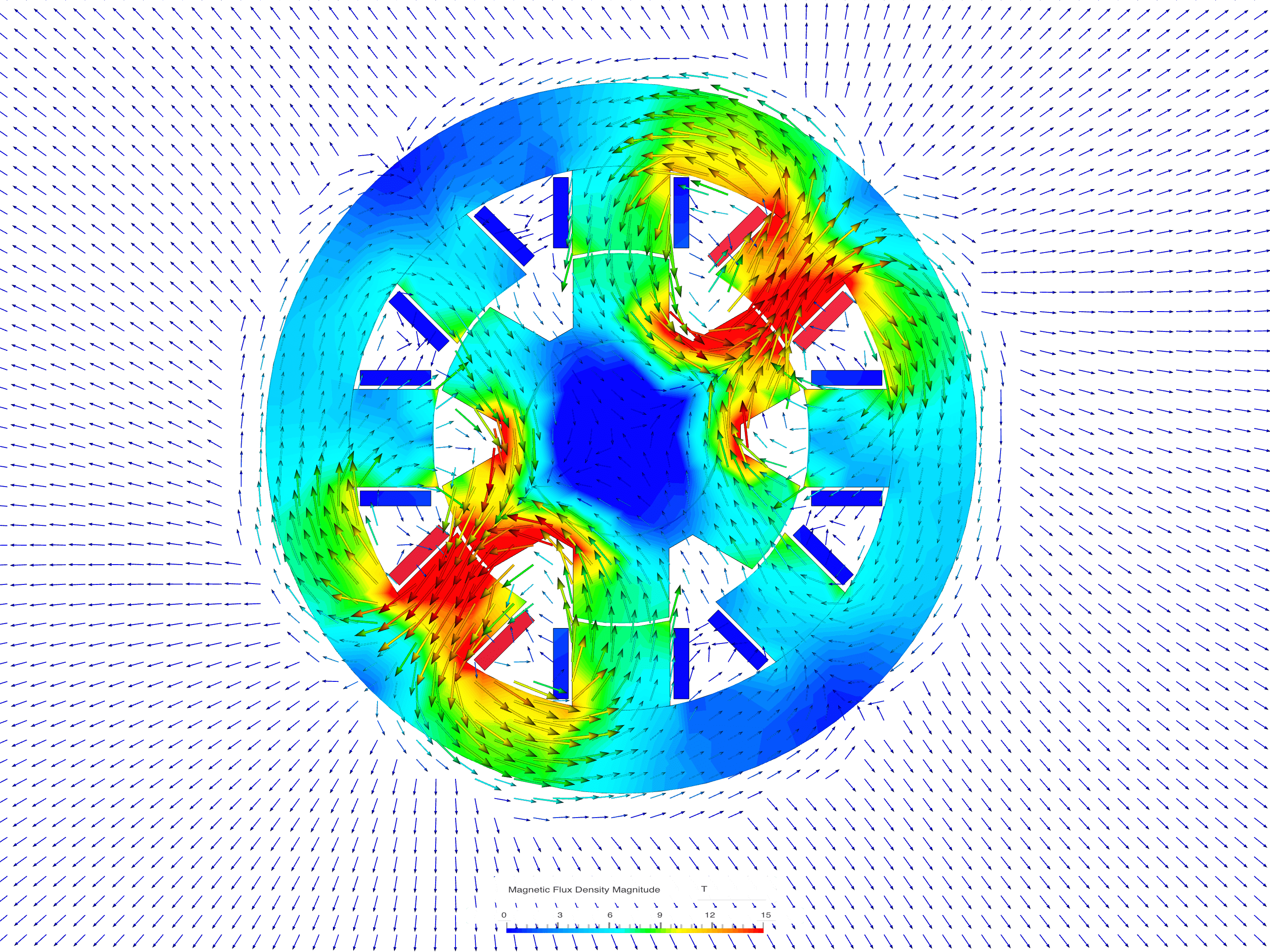
Electromagnetics Analysis
The Electromagnetics (EM) solver aims to provide a powerful tool for simulating electromagnetic phenomena in the cloud. SimScale’s initial focus is centered around static and low-frequency domains along with a steady-state thermal coupling; these solvers help address a major part of electromagnetic devices.
In the near future, we plan to introduce additional modules that will extend the thermal coupling to the transient and electric solvers, coupling with structural mechanics, high-frequency applications, and time-harmonic electrics.
The following information will explain the step-by-step procedure to set up an Electromagnetics simulation within the SimScale platform.
Creating an Electromagnetics Analysis
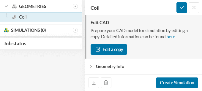
To create an electromagnetics analysis, first, select the desired geometry and click on ‘Create Simulation’:
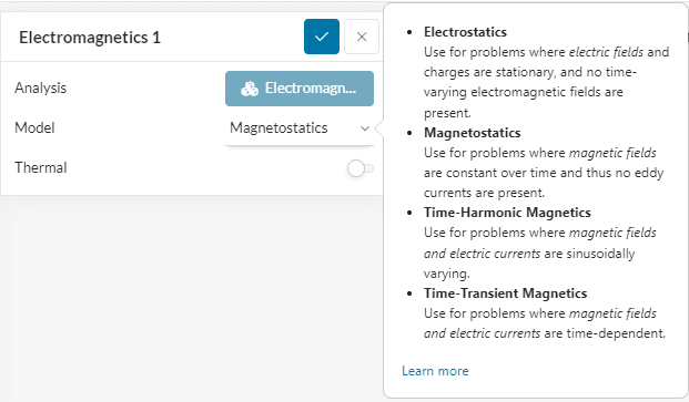
Next, a window with a list of several analysis types supported in SimScale will be displayed:
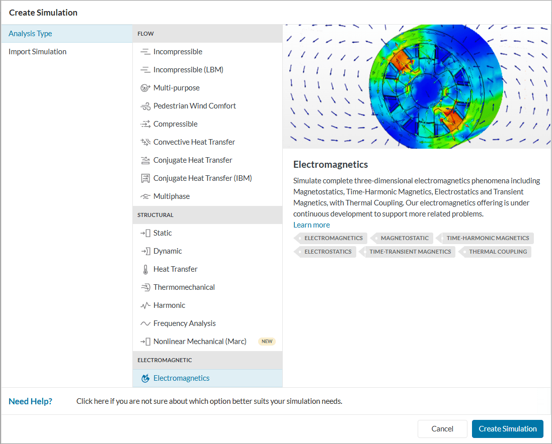
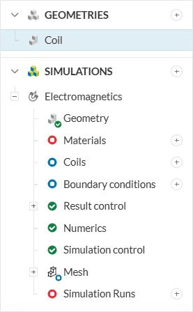
Choose ‘Electromagnetics’ analysis type and click on ‘Create Simulation’. This will open the electromagnetics simulation tree which shows the steps needed to define the simulation.
Global Settings
To access the global settings, click on ‘Electromagnetics’ in the simulation tree. Inside the global settings, you can define the model for your simulation which defines the dominant field of the simulation.
The current capabilities are matured in the low-frequency magnetics simulation domain, providing access to Magnetostatics, which examines static magnetic fields (DC currents) and time-harmonic magnetics for modeling electromagnetic induction phenomena.
For those two solvers a direct coupling to a steady-state thermal conduction solver is available. Where the thermal problem is solved for temperature by considering electromagnetic losses such as ohmic, core losses, and displacement losses.
Moreover, the Time-Transient magnetics solver provides a robust and efficient way to simulate varying magnetic fields in time, e.g. due to a pulse current or voltage.
In regards to electric solvers, SimScale currently provides support for an Electrostatic solver which can be used for the study of electric fields, charges, and their interactions in electrostatic equilibrium and capacitance matrix calculation.
Geometry
The Geometry section allows you to view and select the CAD model required for the simulation. It is important that the CAD model is well-prepared to avoid any meshing or simulation-related errors. Find more details on CAD preparation and upload here.
Materials
In this step, users can define materials based on the material properties relevant to the analysis type chosen for the simulation. SimScale offers a default material library that enables a convenient and quick selection of materials. Additionally, users have the flexibility to create custom materials, which can then be saved in their personal material library for future use.
Magnetic Based Simulation
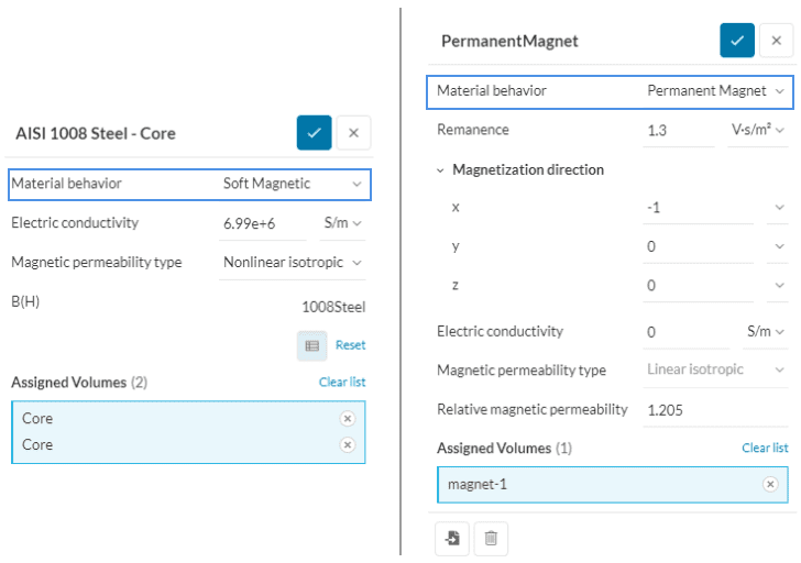
In simulations dominated by a magnetic field (such as Magnetostatics or Time-Harmonic magnetics), the material setup typically follows a consistent pattern. Materials are categorized based on their behavior, which can be either Soft Magnetic or Permanent Magnet.
Both behavior types share common settings, including the material’s electrical conductivity and magnetic permeability. However, Permanent Magnet materials require two additional inputs: the Remanence and Magnetization direction of the permanent magnet.
In a Time-Harmonic Magnetic, and Time-Domain Magnetic simulation, it is possible to additionally define core losses to a material. (Read more in the Core losses section)
In the following, a brief explanation of the terminology used for the material setup is provided.
Soft Magnetic Materials
Soft magnetic materials refer to substances that easily undergo magnetization and demagnetization processes, typically characterized by an intrinsic coercivity of less than 1000 \(\frac{A}{m}\). Intrinsic coercivity refers to the minimum magnetic field strength required to reduce the magnetization of a magnetic material to zero after it has been magnetized, indicating the material’s resistance to losing its magnetization.
These materials are primarily employed to enhance or direct the magnetic flux generated by an electric current. A key parameter for assessing soft magnetic materials is their relative permeability \(\mu_r\), which measures their responsiveness to an applied magnetic field.
Applications for soft magnetic materials can be categorized into two main types: Direct Current (DC) and Alternating Current (AC). In DC applications, the material is magnetized for a specific task and then demagnetized when the task is over. For example, an electromagnet of a lifting machine in a scrap yard is magnetized to attract scrap steel and demagnetized to drop the steel.
In AC applications, soft magnetic materials are repeatedly magnetized in different directions throughout their operational cycles, as seen in devices like power supply transformers. In both DC and AC applications, high permeability is desirable, but the significance of other material properties varies.
For DC applications, the primary consideration in material selection is often permeability, particularly in shielding applications where flux control is essential. Saturation magnetization may also play a role when the material is intended to generate magnetic fields or forces.
In AC applications, minimizing energy losses during the cyclic magnetization process is crucial. These losses can originate from three sources: hysteresis loss (related to the area within the hysteresis loop), eddy current loss (associated with electric currents induced in the material and resistive losses), and anomalous loss (linked to domain wall movement within the material).
Permanent Magnets
Permanent magnets are fundamental components of modern technology, playing a pivotal role in various applications, from electric motors and generators to magnetic storage devices and medical imaging equipment. These materials exhibit a remarkable property: they possess a persistent magnetic field without the need for an external power source. This enduring magnetic field is what sets permanent magnets apart from temporary magnets, which only exhibit magnetic properties when exposed to an external magnetic field.
This property arises from the alignment of magnetic domains within the material, which remains fixed unless subjected to external factors such as high temperatures or strong opposing magnetic fields. Common materials used for permanent magnets include neodymium-iron-boron (NdFeB), samarium-cobalt (SmCo), and ferrite magnets.
Permanent magnets can be defined by switching the material behavior to “Permanent Magnet” as shown in Figure 6 above.
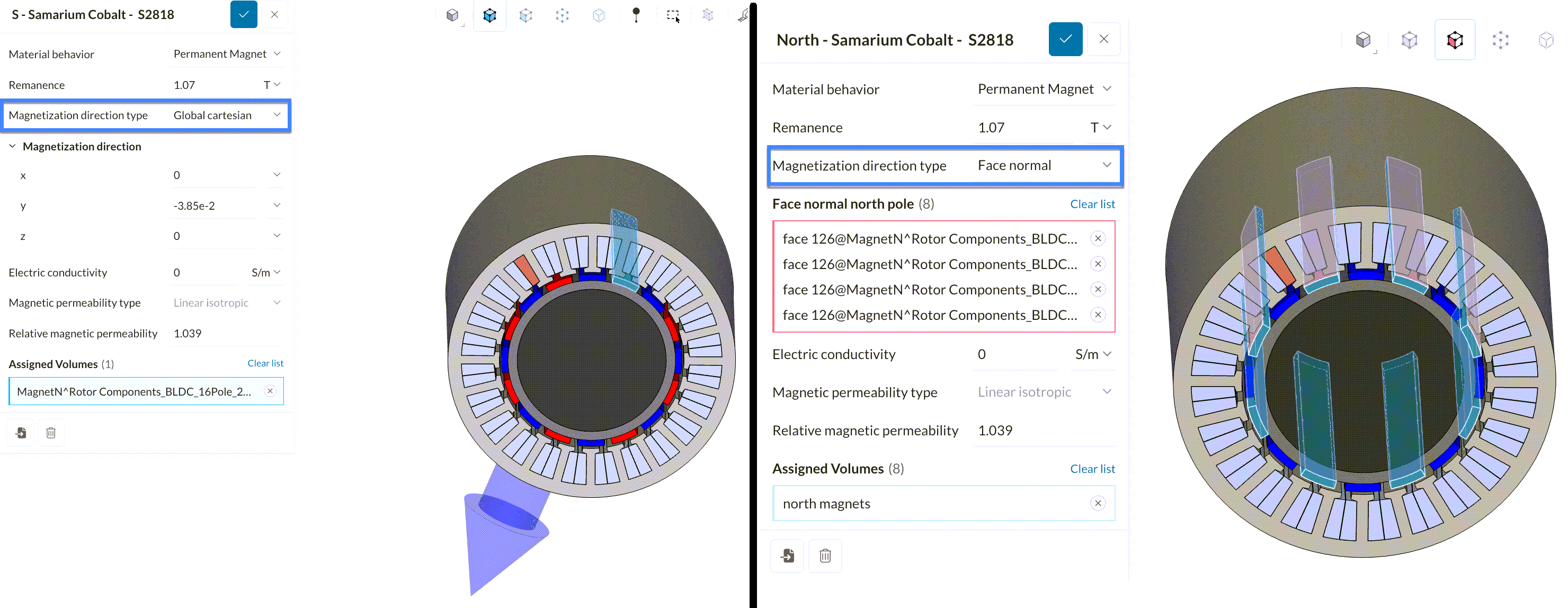
The magnetization direction can be defined in two different ways:
- Global Cartesian: Allows the user to specify custom magnetization vectors based on Cartesian coordinates.
- Face Normal: Enables the user to group multiple magnet volumes (e.g., magnets with north polarization) and align their magnetization vectors with the normal of the selected face. This ensures that the magnetization direction follows the surface normal of the chosen faces.
Orientation and topology of permanent magnets
Currently, the magnetization direction can only be specified based on cartesian coordinates based on the two ways explained above. This implies that the magnetic field emitting from the surface of the permanent magnet is bound to be constant. Simulating permanent magnets with a curved topology (magnetic field tend to concentrate near curved region) will be possible in the near future.
In which simulation models can a permanent magnet be used?
Permanent magnets can be applied in Magnetostatics and Time-Transient Magnetics. However, they cannot be applied in a time-harmonic magnetic simulation. This is because the field generated by permanent magnets is inherently static, whereas in a Time-Harmonic magnetics simulation, the field is fundamentally harmonic.
Magnetic Permeability
Magnetic permeability, denoted by the symbol \(\mu\), is a measure of how easily a material can be magnetized in the presence of a magnetic field. It quantifies the material’s ability to support the formation of magnetic flux within itself when subjected to an applied magnetic field. Materials with high permeabilities allow magnetic flux through more easily than others.
Magnetic permeability is scalar if the medium is isotropic or a 3×3 matrix otherwise. Unlike electrical permittivity, permeability is often a highly nonlinear quantity, especially for steel and iron (ferromagnetic materials).
Mathematically, magnetic permeability is defined as the ratio of the magnetic flux density \(\textbf{B}\) to the magnetic field strength \(\textbf{H}\) within a material:
$$ \mu = \frac{\textbf{B}}{\textbf{H}} $$
Units of Measurement: The SI unit of magnetic permeability is Henry per meter \([\frac{H}{m}]\) or equivalently, Tesla meter per ampere \([\frac{T.m}{A}]\).
Types of Magnetic Permeability:
- Absolute Permeability (\(\mu\)): It represents the magnetic response of a material in isolation and is commonly used to characterize magnetic materials.
- Relative Permeability (\(\mu_r\)): Is a dimensionless quantity that compares the magnetic response of a material to that of free space (or vacuum). It is defined as the ratio of the absolute permeability of the material (\(\mu\)) to the permeability of free space (\(\mu_0\)), often denoted as \(\mu_0\) = 4π × 10⁻⁷ \(\frac{H}{m}\).
$$ \mu_r = \frac{\mu}{\mu_0} $$
Since the permeability is a very small number, the relative permeability is the most commonly used parameter for material definitions.
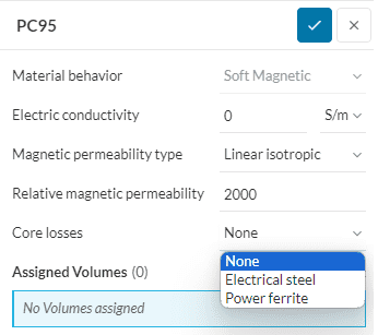
In the setup, the user can choose the ‘Magnetic permeability type’ which can be either Linear Isotropic or Nonlinear Isotropic. In the prior, a constant value of the Relative magnetic permeability is defined, while for the latter a B-H curve can be uploaded.
Figure 8 illustrates a comparison between linear and nonlinear magnetic permeability material definitions.
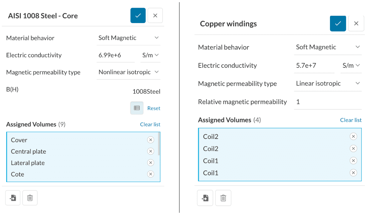
Figure 9 shows the table input for a nonlinear magnetic permeability. The units of \(\textbf{H}\) and \(\textbf{B}\) should be provided in SI units as \(\frac{A}{m}\) and \(T\) or \(\frac{V.s}{m^2}\), respectively.
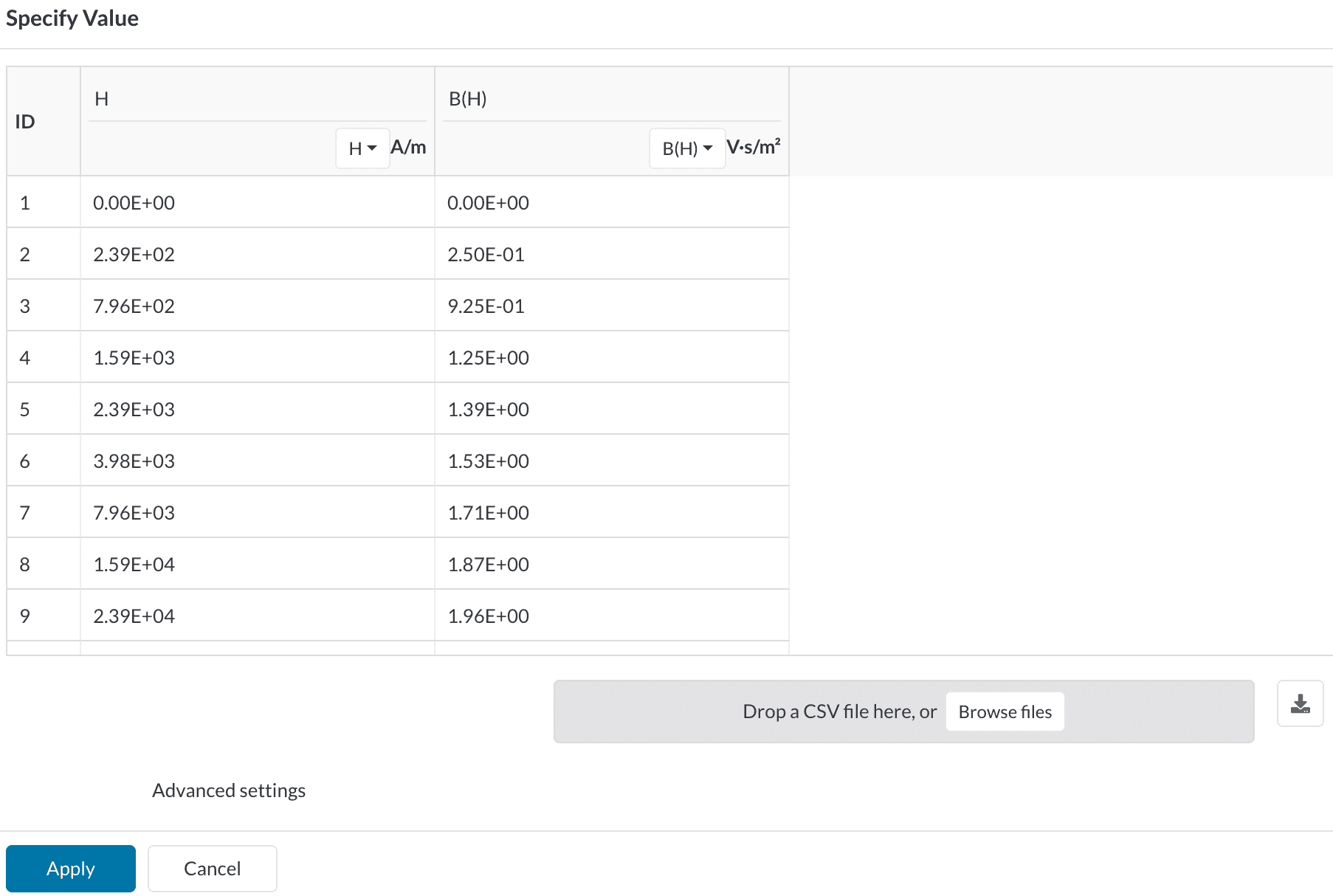
Uploading \(\textbf{B}\)\(\textbf{H}\)-curve data
There are two main rules that need to be satisfied when importing \(\textbf{B}\)\(\textbf{H}\)-curve data:
Electric Permittivity
Electric permittivity, also known as dielectric constant, is a fundamental property of materials that describes a measures of the electric polarizability of a dielectric material. It is denoted by the symbol \(\epsilon\) and it quantifies how easily electric charges can move through or be displaced within a material when subjected to an electric field.
A substance exhibiting high permittivity reacts more intensely to an applied electric field compared to one with lower permittivity, consequently accumulating greater energy within the material. Within electrostatics, permittivity serves as a critical factor in defining the capacitance of a capacitor.
Electric Permittivity is a coefficient that links the strength of the electric field within a material to the level of electric displacement in that material. The electric displacement field \(\textbf{D}\) represents the arrangement of electric charges within a specified medium triggered by the existence of an electric field \(\textbf{E}\). This arrangement encompasses both the migration of charges and the reorientation of electric dipoles.
In the simplest case involving linear, homogeneous, isotropic materials with an “instantaneous” reaction to alterations in the electric field, its correlation with permittivity is given as:
$$ \textbf{D} = \epsilon \textbf{E} $$
Where
\(\textbf{D}\) is the electric displacement \([\frac{C}{m^2}]\),
\(\textbf{E}\) Electric field \([\frac{V}{m}]\),
and \(\epsilon\) is the electric permittivity \([\frac{F}{m}]\).
The dynamics between charged objects are defined by the interplay of \(\textbf{D}\) and \(\textbf{E}\). \(\textbf{D}\) is related to the charge densities involved in this interaction, while \(\textbf{E}\) is related to the forces at play and the potential differences.
The permittivity is often represented by the relative permittivity \(\epsilon_r\) which is the ratio of the absolute permittivity \(\epsilon\) and the vacuum permittivity \(\epsilon_0\) which has a value of \(\epsilon_0\) = 8.85×10⁻¹² \(\frac{F}{m}\):q
$$\epsilon_r = \frac{\epsilon}{\epsilon_0}$$
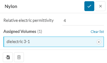
Electric permittivity as a material property is only required in an Electrostatic analysis, and in fact, it is the only material property relevant for this analysis type. Electric conductivity is not required because it is considered either infinite in conducting objects or zero in insulators.
For an Electrostatic analysis, each component or body must be assigned a relative electric permittivity. This quantity is a real number larger than or equal to 1.0 for isotropic materials.
Remanence
Remanence (\(B_r\)) also known as retentivity or residual magnetism is a fundamental concept in the field of magnetism and materials science that describes the phenomenon whereby certain materials retain a permanent magnetization even after an external magnetic field is removed. This enduring magnetization arises from the alignment of magnetic moments within the material’s atomic or molecular structure. In simple terms, the higher the value of Remanence the stronger the magnet is.
For example, the magnetic memory in magnetic storage devices, as well as in everyday magnets or materials that can be easily magnetized, is a result of remanence. When there is a need to eliminate this remanence, it can be accomplished by subjecting the material to a negative inducing field, a procedure commonly referred to as degaussing.
The concept of remanence can be easier to understand through the magnetic hysteresis curve shown in Figure 11 below. The hysteresis curve illustrates the relationship between the magnetic field strength \(\textbf{H}\) and the resulting magnetic induction \(\textbf{B}\) in a material, showing how a material responds as it is magnetized and demagnetized.
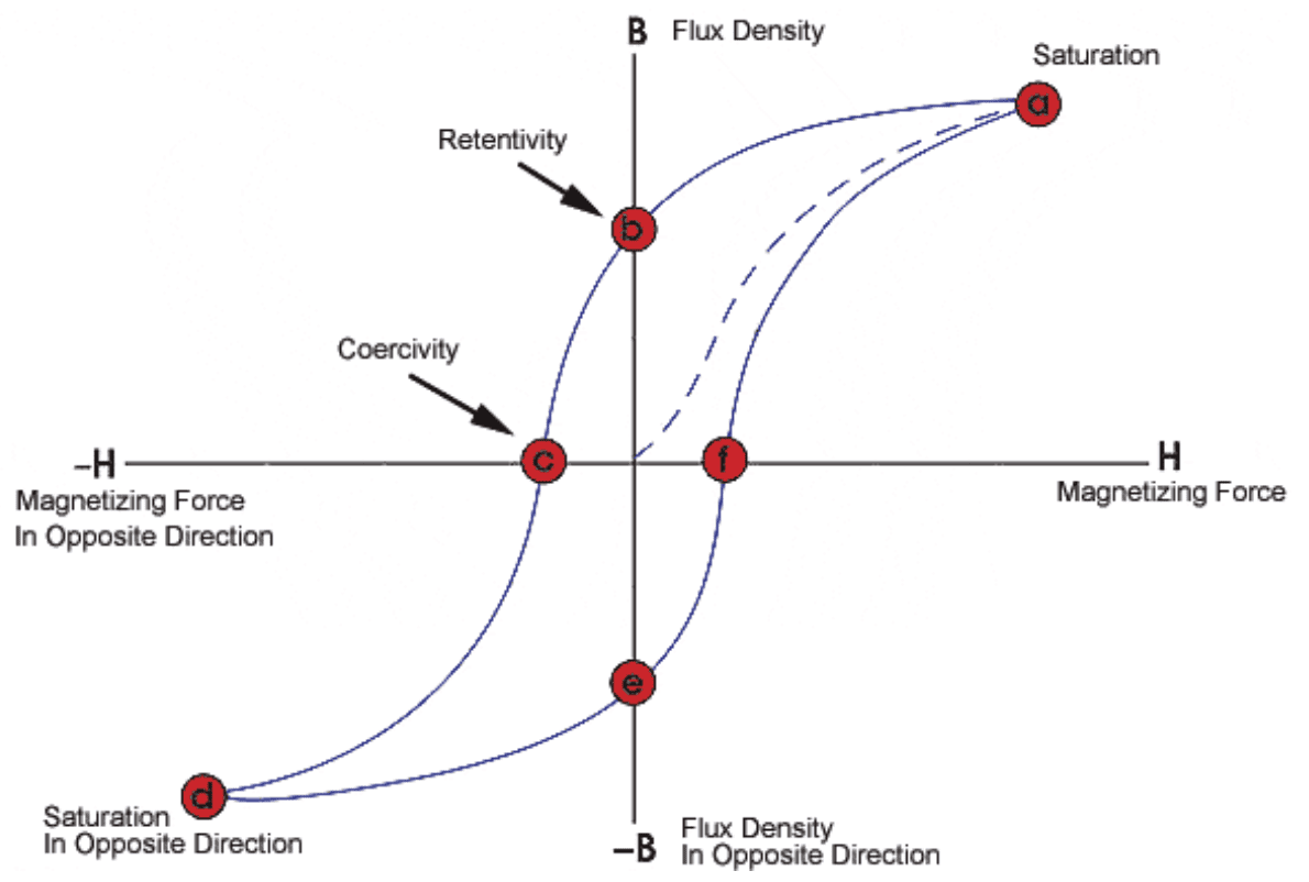
In the case of a ferromagnetic material that has never been magnetized before or has been completely demagnetized, it will follow the dashed line when \(\textbf{H}\) is increased. This line shows that the higher the applied magnetizing force or current (\(\textbf{H}\)+), the stronger the magnetic field within the component (\(\textbf{B}\)+).
At point “a” almost all of the magnetic domains are aligned, and further increase in the magnetizing force will result in minimal additional magnetic flux. This marks the material’s state of magnetic saturation.
When \(\textbf{H}\) is reduced to zero, the curve shifts from “a” to “b.” At the intersection of the curve with point “b”, it’s evident that some residual magnetic flux \(\textbf{B}\) remains within the material despite a zero magnetizing force. This point is known as remanence or retentivity on the graph and signifies the material’s remanence or the degree of remaining magnetism (where some domains maintain alignment while others lose it).
As the magnetizing force is reversed, the curve progresses to point “c,” where the flux is reduced to zero. This is termed coercivity on the curve, indicating that the reversed magnetizing force has flipped enough domains to nullify the net flux within the material. The energy required to eliminate the remaining magnetism from the material is referred to as the coercive force or coercivity of the material.
Hard and soft magnetic materials on a hystersis curve
Typically, hard magnetic materials are commonly referred to as permanent magnets, and these materials exhibit a B-H Curve that commences in the second quadrant when displaying nonlinear behavior. On the other hand, there are magnets, distinct from permanent magnets, known as soft magnetic materials, whose B-H Curve is confined to the first quadrant.
Electrical conductivity
Electrical conductivity, also known as specific conductance or simply conductivity, refers to the ability of a material to conduct an electric current. It is a fundamental property of materials that determines how easily electric charges can flow through them. Conductivity is typically measured in units of Siemens per meter \([\frac{S}{m}]\)
In a solid material, electrical conductivity is influenced by the movement of charged particles, such as electrons or ions. Metals are excellent conductors of electricity due to the presence of free electrons that are loosely bound to the atomic structure. When a potential difference (voltage) is applied across a metal, these free electrons can move freely and carry the electric charge, resulting in high conductivity.
In contrast, insulators have very low electrical conductivity because their electrons are tightly bound to the atomic structure, making it difficult for them to move. Examples of insulators include plastics, rubber, glass, and ceramics. These materials impede the flow of electric current, and their conductivity is typically negligible for practical purposes.
Semiconductors, however, have an intermediate level of conductivity that can significantly vary depending on factors such as exposure to electric fields or specific frequencies of light
Electrical conductivity finds application in analyses such as Electric Conduction, AC Magnetic, and Transient Magnetic studies.
Core Losses
Available in a Time-Harmonic Magnetic simulation. Core losses also known as iron losses, are a critical consideration in electromagnetic simulations, particularly in devices like transformers and inductors. These losses occur within the magnetic core material due to two primary mechanisms: magnetic hysteresis and eddy currents.
Magnetic hysteresis refers to the phenomenon where a material retains some magnetization even after the magnetic field causing it has been removed. When the magnetic field reverses direction, the material must undergo a certain amount of energy loss to realign its magnetic domains. This energy loss manifests as heat within the core material and is known as hysteresis loss.
Eddy currents, on the other hand, are induced currents that circulate within the bulk of the core material due to changing magnetic fields. These currents result in resistive losses within the core material, converting part of the electromagnetic energy into heat.
SimScale supports two different models for calculating core losses depending on the type of material used.
1. Electrical Steel:
For modeling losses in a laminated core, consisting of thin layers of insulated electrical steel designed to minimize eddy current losses.
Losses are calculated using Bertotti’s model. Which is based on a separation of the types of losses (hysteresis, eddy currents, and excess losses), the Bertotti model computes the losses using the following parameters:
$$ \rho W_c = K_h f B_m + K_c f^2 B^2 + K_e f^{1.5} B^{1.5} $$
where \(K_{h}\) is the hysteresis loss coefficient, \(K_{c}\) is the eddy current loss coefficient, and \(K_{e}\) is the excess loss coefficient, \(f \) is the frequency and \(\textbf{B}\) is the magnetic flux density.
2. Power Ferrite:
For modeling losses in a ferrite core, which is a ceramic compound composed of iron oxide mixed with other metallic elements, characterized by high magnetic permeability and low electrical conductivity. Losses are calculated using the Steinmetz formula:
$$ \rho W_c = K_s f^{\alpha} B^{\beta} $$
where \(K_s\) is the Steinmetz constant, \(\alpha\) is the frequency exponent, and \(\beta\) is the flux density exponent.
Eddy currents and Core loss models
When a core loss model other than None is enabled, eddy currents are suppressed in that body.
Coils
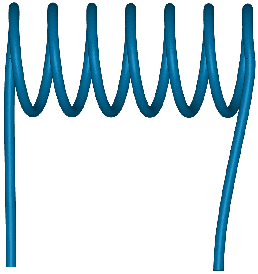
A coil is a configuration where the length of the conductor, often copper wire, is wound multiple times around a central core. When an electric current flows through these windings, they collectively generate a magnetic field. This phenomenon forms the basis for various applications in electromagnetics.
Solid and Stranded Coils
In the context of coils, a notable distinction is drawn between two main categories: Solid coils and Stranded (wound) coils.
A Solid coil is crafted from a single continuous piece of conductor material, providing an unbroken path for electric current. As the current flows through this uninterrupted path, the current density—defined as the amount of current per unit cross-sectional area—can vary based on the conductor’s geometry. In Solid coils, irregularities in the conductor’s material or variations in its cross-sectional dimensions can lead to uneven current distribution and subsequently non-uniform current density.
Conversely, a stranded coil refers to a volume modeling of a coil that is formed by wrapping multiple turns of a conductor, typically made of materials like copper wire, around a cylindrical core or bobbin. A Stranded coil definition allows the user to simplify the modeling approach of the actual stranded coil, by simply replacing the stranded coil wires with an equivalent size cross-section.
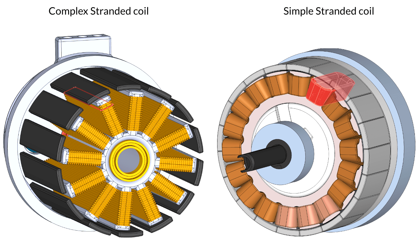
For example, Figure 14 below highlights the difference in modeling approaches between a complex and a simple stranded coil approach. In this example, two different electric motor geometries are shown. Where one is modeled with actual strands of wire, and in the other approach these strands are lumped together into an equivalent volume, in which later in the simulation setup the number of turns of the wire inside that volume would be specified.
Utilizing the Stranded coil type definition not only simplifies the geometry creation process but also leads to a reduction in both mesh element count and simulation computation time. This approach allows for the creation of a single or multiple-volume coil that mimics the behavior of being stranded, hence eliminating the need for manual strand-by-strand construction.
Moreover, if one were to go ahead with the complex stranded coil approach, then each strand of wire would need to be defined as a coil. In that case, the coil could be either defined as a solid coil, or a stranded coil with 1 turn. However, since there is a large number of coils that need to be defined, the complex approach would be significantly more time-consuming to set up than the simple stranded coil approach.
Moving on, the distinct current distribution in these coil types influences the resulting magnetic field. In a solid coil, the uneven current density can lead to non-uniform magnetic field generation, with stronger magnetic effects where the current density is higher and weaker effects where it’s lower. In contrast, the uniform current density in a Stranded coil produces a magnetic field that is generally more evenly distributed and consistent.
The total current flowing in a Stranded coil is simply the current per turn multiplied by the total number of turns: \(I = \frac{current}{turn} * N\)
In the case of a Solid coil, the total current is simply the net current \(I\) flowing through it. This means that in both stranded and solid coils, the net current would be the same in the end. If that is the case, one may wonder what is really the difference between solid and stranded coils when it comes to their applications in simulations.
The disparities between these coil types emerge based on the chosen type of analysis. Whether it involves Magnetostatic, Time-harmonic magnetics or Time-transient magnetics simulations, the distinctions become apparent.
In the study of Magnetostatics, there are no induced currents, and hence the total current in the coil is simply the applied current. As previously mentioned, the current density distribution in a stranded coil is uniform, however, it varies in a solid coil. Consequently, there can be a small difference in the magnetic field between the two. Inductances, on the other hand, would be completely different between solid and stranded coils since it depends on the number of turns.
In Time-Harmonic Magnetics studies, it’s crucial to distinguish between stranded and solid coils. In a stranded coil, the diameter of each wire turn is typically much smaller than the Skin Depth, and individual turns are insulated from each other. As a result, stranded coils do not facilitate the flow of Eddy Currents, which are induced currents. Conversely, in a solid coil, the conductor’s size is usually larger than the Skin Depth, allowing Eddy currents to flow. Eddy currents typically move in the opposite direction to the applied current in the coil.
Litz Wire
Litz wire is another coil type available for use in SimScale. This type of coil is commonly employed in power-conversion equipment as a way to reduce alternating-current (AC) losses in conductors.
A Litz wire bundle is composed of multiple insulated strands or filaments, each electrically isolated from the others but connected in parallel or continuously twisted together. The bundle maintains nearly the same direct-current (DC) resistance and effective current-carrying area as a single solid wire.
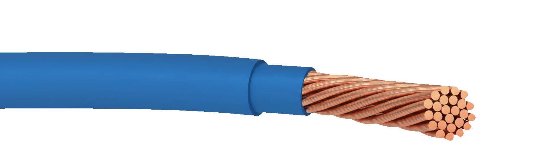
Because each individual strand has a diameter smaller than one skin depth, it experiences negligible skin-effect losses. As a result, AC losses, both skin effect and proximity effect, are significantly reduced compared to a single solid conductor of the same cross-section.
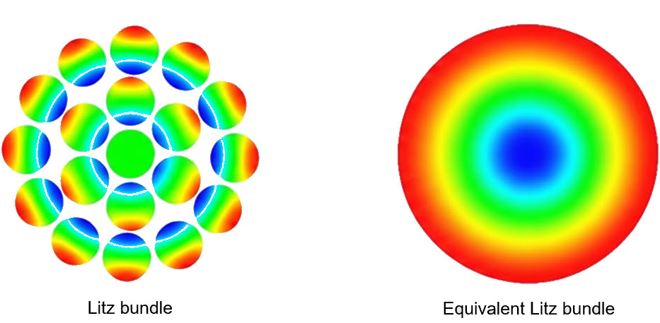
In SimScale, instead of explicitly modeling the hundreds or thousands of strands that may exist in a real Litz bundle, it can be represented geometrically as a single object with the same outer diameter, as shown in the figure below.
Setting Up a Coil
The setup of coils in SimScale revolves around two fundamental parameters: Coil type and Topology. These parameters determine how your coil will behave in the simulation.
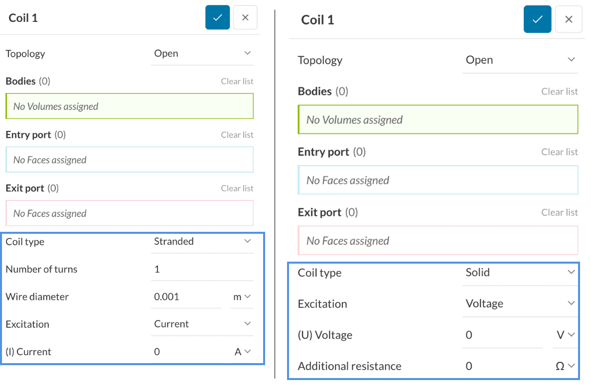
Coil type
The Coil type parameter classifies coils into three categories: Solid, Stranded and Litz Wire. This classification defines the coil’s structural composition and its subsequent behavior within the electromagnetic field.
In a Solid coil only the Excitation needs to be defined, which can either be via a net (I) Current or a (U) Voltage, while for a Stranded coil, two additional parameters to the Excitation are required, which are the Number of turns and Wire diameter.
- Excitation:
- Magnetostatics:
- (I) Current: For a solid coil it is the net current flowing through the coil. For a stranded coil, the current per turn should be specified.
- (U) Voltage: The voltage across the coil ports is to be specified; an Additional resistance value can also be added to the voltage definition.
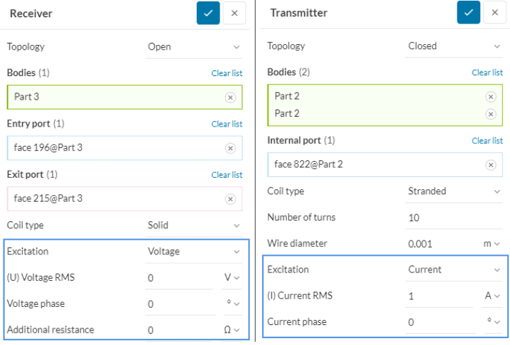
- Time-Harmonic Magnetics:
- For both the current and the voltage: The magnitude of the RMS current or voltage and the associated phase are to be specified.
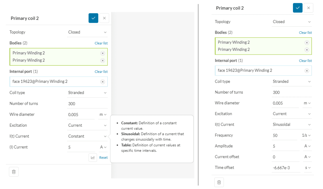
- Time-Transient Magnetics:
- Constant: Similar to Magnetostatics and Time-Harmonics, the user can define a constant current or voltage excitation.
- Sinusoidal: Define a sinusoidal current or voltage signal that varies in time. Input parameters are Frequency, Amplitude, Current offset, and Time offset. The time offset can be used to define the signal’s phase shift in time.
- Table: Specify a function curve that gives the peak current or voltage as a function of time. It can be used for example to define an input pulse.
- Magnetostatics:
- Number of turns: This is the number of turns of a wire around a core or bobbin.
For example, if you have a wire that has a bundle of 4 strands that is winded 50 times around a core, then the number of turns would be 50 and not 200. - Wire diameter: The diameter of the round wire cross-section.
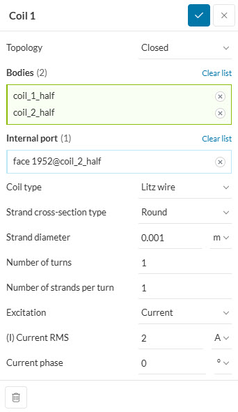
Setting Up a Litz Wire Coil
This option shares common fields for the Excitation, however, there are other parameters that needs to be set with the aim to define the litz wire:
- Strand cross-section type: The ratio between the volume actually occupied by the winding and the total volume available to contain it (fill factor). Because conductors always leave small gaps and require insulation between turns and layers, the fill factor is always less than one. It is defined as the ratio of the conductor’s cross-sectional area to the total coil cross-sectional area. For example, a fill factor of 0.9 means that 90% of the area is conductor and 10% is insulation or gaps. SimScale offers two options for defining the type of cross-section for strands:
- Round Wire: For a round wire shape, the filling factor for a Litz wire winding type with\(N_{s}\) strands and \(N_{T}\) turns is computed as follows: $$ F=\frac{N_S N_T d^2}{4 A} $$ \(N_{s}\) is the number of strands, \(N_{T}\) is the number of turns, d is the diameter of the round wire section and A is the total cross section area of the coil.
- Square Wire: For a square wire shape, the filling factor is computed as follows: $$ F=\frac{N_S N_T w^2}{A} $$ \(N_{s}\) is the number of strands, \(N_{T}\) is the number of turns, w is the edge width of the square wire section and A is the total cross section area of the coil.
- Strand diameter: Size of the individual, insulated wire that is twisted together with other strands to form the final conductor;
- Number of strands per turn: The design parameter specifying how many elements (individual strands or sub-bundles) are grouped and twisted together at a given stage of the Litz wire.
Specifying current for multiple coil bodies in one coil setup
The current value specified for in a coil setup is averaged over the number of coil bodies inside that setup. For example, if you have a coil setup which has 4 coils defined inside it, meaning 4 entry and 4 exit ports or 4 internal ports. Then if the input current is 100 Amperes, this would result in each coil receiving a current value of 25 Amperes. If the intended current in each of the 4 coils was 100 Amperes, then the value given inside the coil setup should be 400 Amperes.
Parametric simulations
In the simulation, the current input is parameterizable. With parametric studies, the user can quickly set up, run, and compare results for several configurations in parallel saving heavily on computational time. Currently, SimScale supports only one parametric definition in the simulation seutp. Meaning, you would not be able to parametrize the current inputs for multiple coils.
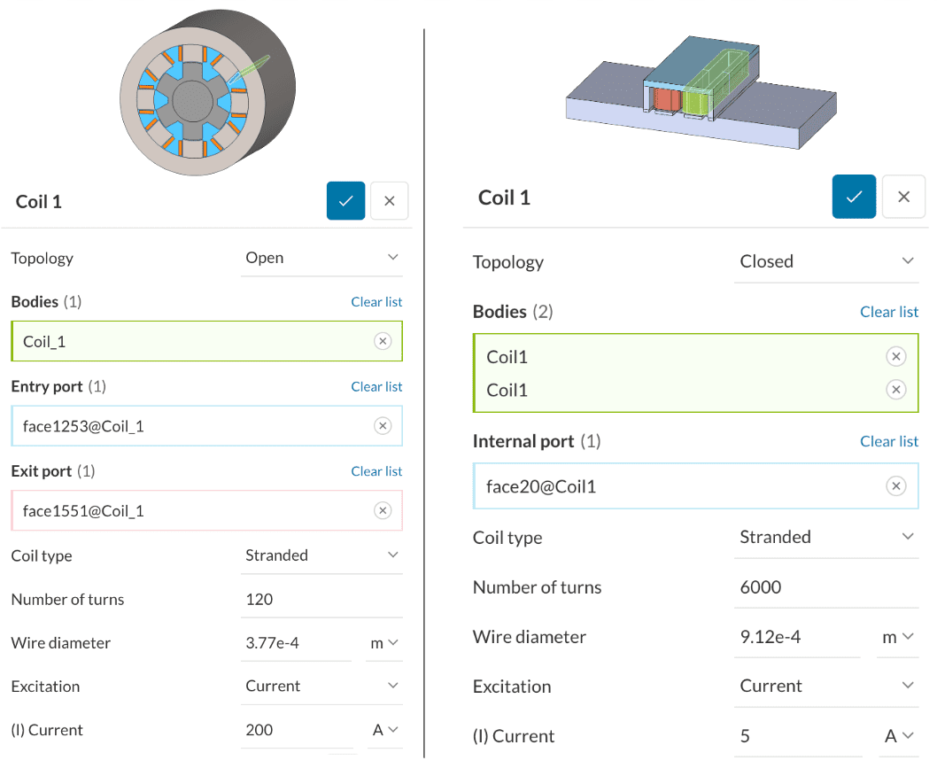
Topology
The Topology parameter dictates whether your coil is characterized as Open or Closed. This defines whether the coil is modeled as a closed loop or has open boundaries.
In general, The net current does not give information about the direction of current flow in the coil. It is the current density that gives such information. Therefore, it is necessary to specify a port or a pair of ports that dictates the direction in which the current flows.
- Closed Topology: The coil forms a complete loop, meaning that the entire coil circuit is modeled as a connected loop. Here an Internal port must be defined.
Defining closed loop coils requires consideration at the geometry level. A planar inlet made up of one or multiple surfaces, where current density flows perpendicular to the inlet, must be made reachable. This can be achieved by splitting the coil into two or more parts in order to have access to an internal face. - Open Topology: The coil has an open topology which means it has two clear ends. Here an Entry port and an Exit port must be defined.
These ports must be planar and can be made up of many faces. The current density flows orthogonally into the Entry Port and out of the Exit Port. Thus the port specification gives the direction of the current flow
Figure 18 below compares the setup of an open coil (left) to the setup of a closed coil (right). Notice, in the open coil scenario, the coil has an open topology with clear entry and exit ports on the front and back sides of the motor. On the other hand, an internal port is chosen for the closed coil.
Boundary Conditions
Boundary conditions help to add closure to the problem at hand by defining how a system interacts with the environment.
Depending on whether the simulation is based on a magnetic dominant field or an electric dominant field, the boundary conditions associated with that particular analysis can vary.
Magnetic Field Simulations
Two types of boundary conditions are supported in the context of a magnetic dominant field analysis type (e.g. Magnetostatics, Time-Harmonic Magnetics) that aid in fully defining the problem at hand.
These are the Magnetic Field Normal and Magnetic Flux Tangential:
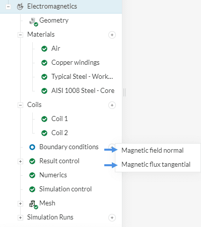
Magnetic Field Normal
This boundary condition enforces the presence of a normal magnetic field \(\textbf{H}\), effectively nullifying any tangential magnetic field \(\textbf{H}\), across a given surface. The normal field must be applied on all faces belonging to a plane of symmetry where the magnetic field \(\textbf{H}\) is purely normal.
Magnetic Flux Tangential
This boundary condition enforces the presence of tangential flux, effectively nullifying any normal flux \(\textbf{B}\), across a given surface. The Tangential flux must be applied on all faces belonging to a plane of symmetry where the magnetic flux density is purely tangential.
If a coil is in contact with the bounding box (e.g. air volume) boundary and if the current is flowing normal to that boundary, then a tangential flux boundary condition must be applied. In other words, if you have an entry or an exit port that is aligned with the outer boundary of the bounding box then assign a tangential flux boundary condition on all the faces on that boundary.
- The reason behind this is due to Maxwell-Ampere’s law which states that the circulation of the magnetic field \(\textbf{H}\) around a closed path equals the current flowing through the surface bounded by that path. Based on this, let’s take the scenario where a normal field boundary condition would be assigned instead of an external boundary where a current flows through:
- The normal field boundary condition enforces that the tangential component of the magnetic field \(\textbf{H}\) is zero, and integrating that field over a path that encloses the boundary of the coil would also be zero, which contradicts Maxwell-Ampere’s law.
Note that when applying those boundary conditions they should be assigned on all faces of the external boundaries.
Why are the boundary conditions called Magnetic flux tangential and Magnetic field normal?
Simply because that is exactly what is prescribed in the equations. In the magnetic flux tangential BC the normal component of the magnetic flux density is zero, and in the normal field BC the tangential component of the magnetic field is zero. Useful to know is that, for an isotropic material the flux tangential BC also means that the field is tangential, and the field normal BC also means that the flux is normal. However, in general (for anisotropic materials) this is not true. Hence, the naming is as such in order to maintain an accurate representation of the names.
Electric Field Simulations
This relates only to the Electrostatics analysis type. Below a description of each of the available boundary conditions is provided.
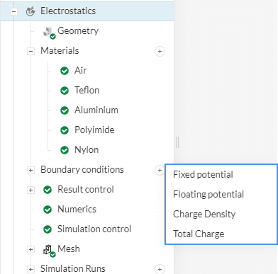
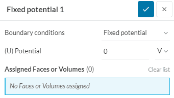
Fixed Potential
The fixed voltage boundary condition imposes a voltage on a face or a volume. All the nodes of the restrained face or volume are assigned the specified voltage.
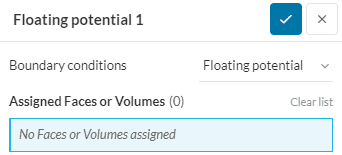
Floating Potential
The floating potential constraint implies an unspecified voltage value. It is treated differently depending on whether the capacitance matrix is computed or not.
- If the capacitance matrix is requested, the simulation assigns 1.0 or 0 \(V\) on the entity with a floating potential and computes the matrix using the stored electric energy.
- On the other hand, if the capacitance matrix is not requested, the floating potential entity is treated as an equipotential entity with an unknown voltage value, and thus solved for. Consequently, to treat the voltage on a floating potential entity as unknown, the capacitance matrix shall not be requested.
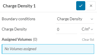
Charge Density
This condition permits imposing a uniform charge distribution on a component or body. The charge density is given in Coulombs per meter cubic \([\frac{C}{m^3}]\).
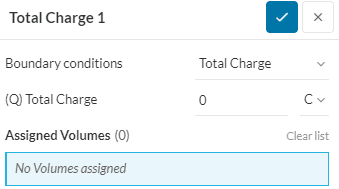
Total Charge
The total charge condition imposes a uniform charge distribution on a volume. The total charge is given in Coulombs \([C]\).
Thermal coupling
The boundary conditions below are accessible once the thermal coupling toggle is activated in the global simulation settings for both: Magnetostatics and Time-Harmonic Magnetics. Below a description of each of the available boundary conditions is provided.
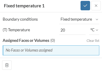
Fixed temperature
The Fixed Temperature boundary condition specifies that a surface, face, or volume within the simulation domain is held at a constant temperature throughout the simulation. This is used to simulate surfaces or regions that are thermally controlled or attached to a heat source or sink with a known temperature. It serves as a thermal constraint, ensuring that any heat transfer processes or thermal effects do not affect the temperature at the specified boundary, which remains fixed regardless of the surrounding conditions.
The Fixed Temperature boundary condition maintains a constant temperature on a selected surface or volume throughout the simulation. It represents a region with a controlled temperature, unaffected by surrounding thermal effects.
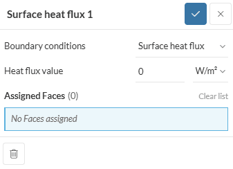
Surface heat flux
The Surface Heat Flux boundary condition specifies the rate of heat transfer through a given surface, measured in terms of energy per unit area per unit time (W/m²). This boundary condition is used to simulate scenarios where heat is actively being added or removed from a surface, such as through convection, radiation, or conduction. The applied heat flux can represent thermal sources, like heaters, or sinks, like cooling devices, and it influences the thermal distribution within the simulation domain based on the magnitude and direction of the heat transfer.
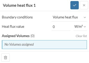
Volume heat flux
The Volume Heat Flux boundary condition defines the rate of heat generation or absorption per unit volume within a material, typically measured in watts per cubic meter (W/m³). This is used to simulate internal heat sources, such as resistive heating from electrical currents, or energy absorption due to radiation or chemical reactions. It affects the overall temperature distribution within the volume by adding or removing thermal energy from the material.
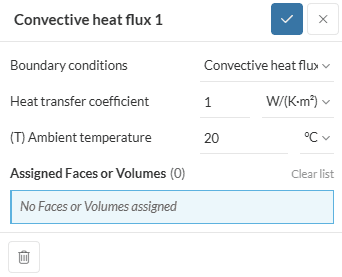
Convective heat flux
The Convective Heat Flux boundary condition models heat transfer between a surface and a fluid (such as air or water) via convection. It is governed by the heat transfer coefficient (W/(m²·K)) and the ambient temperature of the surrounding fluid. This boundary condition simulates the heat exchange due to fluid flow, where heat is transferred from the surface to the fluid or vice versa, depending on the temperature difference. It’s commonly used in scenarios like cooling or heating of objects exposed to airflow or other fluids.
In our workflow, the convection boundary condition is applied directly to the air volume, not to its outer surfaces. This approach is specifically designed to support EM–Thermal coupled simulations efficiently and consistently. Internally, the air region is excluded from the thermal solution — no temperature is computed inside it.
Instead, the convection BC is automatically transferred to all faces of the solid regions that are in contact with the air volume. These faces receive the convection condition using the specified heat transfer coefficient (HTC) and ambient temperature.
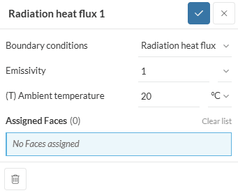
Radiation heat flux
The Radiation Heat Flux boundary condition models heat transfer between a surface and its surroundings via thermal radiation. It accounts for the emission and absorption of radiant energy, based on the surface temperature and the ambient environment, typically using the Stefan-Boltzmann law. This boundary condition is crucial when simulating heat exchange in environments where radiation plays a dominant role, such as in high-temperature systems or when surfaces are exposed to significant radiant energy, like sunlight or furnaces.
Advanced Concepts
Motion Coupling
SimScale enables transient electromagnetic simulations that account for the movement of components such as rotors, magnets, and plungers. Mechanical motion is coupled with electromagnetic field calculations at each time step, allowing accurate analysis of how moving parts interact with magnetic fields, including dynamic effects such as back-EMF, time-varying forces, and torque ripple.
Typical applications include electric motors, solenoids, actuators, electromagnetic sensors, and electromagnetic valves. This feature is available only for the Time-Transient Magnetics solver.
Note
In the current release, only Rotational motion with Prescribed motion mode is supported. Linear (translational) motion and Computed motion mode will be available in a future release.
Overview
When motion coupling is enabled, the simulation domain is divided into three region types:
| Region Type | Description |
|---|---|
| Static | Components that do not move, such as stators and housings. Their mesh remains fixed throughout the simulation. |
| Moving | Components undergoing rigid body motion, such as rotors or permanent magnets. Their mesh is rigidly transformed at each time step. |
| Remeshed | Region surrounding the moving parts that is dynamically remeshed at each time step to maintain a conformal mesh between static and moving regions. |
The Remeshed region is a required part of the setup. It must fully enclose all moving components and must not overlap with static solid bodies.
Setting Up Motion Coupling
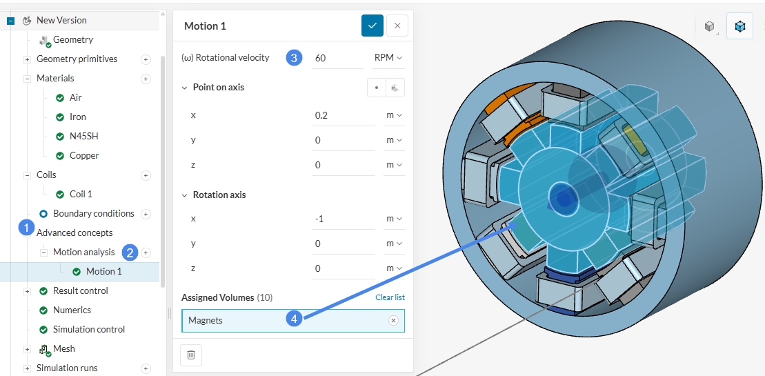
Motion coupling is configured under Advanced Concepts in the simulation tree of a Transient electromagnetic analysis. To add a motion coupling definition:
- In the simulation tree, navigate to Advanced Concepts and select Motion Analysis.
- Click Add Motion to create a new motion definition.
- Specify the rotational velocity and direction.
- Assign the moving geometry volumes to the motion definition.
Motion Type
The Motion Type defines the kind of mechanical movement applied to the selected components. Currently, Rotational motion is supported.
Rotational Motion
Rotational motion applies a continuous angular displacement to the assigned moving volumes around a user-defined axis. This setup is suited for electric motors, rotating magnets, and similar devices.
Define the following parameters for rotational motion:
| Parameter | Description |
|---|---|
| Rotation Axis Origin | A point on the rotation axis, defined by its X, Y, and Z coordinates. |
| Rotation Axis Direction | A vector defining the orientation of the rotation axis (e.g., [0, 0, 1] for the Z-axis). |
| Rotational Velocity | The rotational speed of the moving body, specified in revolutions per minute (RPM) or radians per second. |
Material Requirements
All solid bodies involved in a motion-coupled simulation must have Density defined in their material properties. This applies to both static and moving solid components. Density is required for the computation of inertial effects and force quantities.
Important
If Density is not assigned to a material used in a motion-coupled simulation, the simulation setup will be incomplete. Ensure all materials assigned to moving and static solid bodies include a density value.
Result Control
The Result Control section enables users to define additional simulation result outputs crucial for design analysis. These outputs vary depending on the simulation model (e.g dominant field chosen for the electromagnetic simulation). They can be categorized into user-defined outputs and automatically provided outputs, essential for a comprehensive analysis.
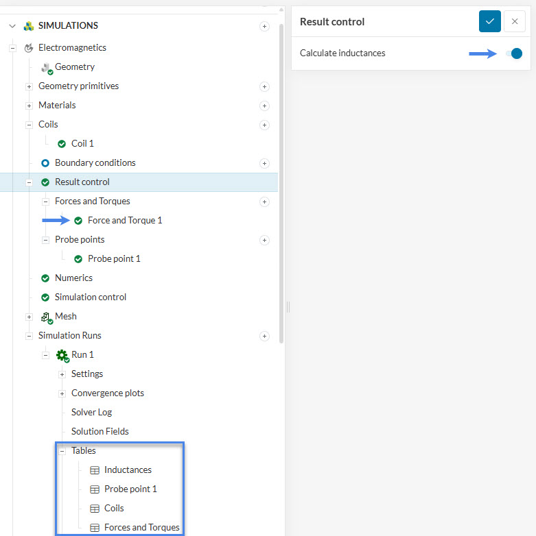
Post-simulation, these result control outputs are presented in table format and can be accessed collectively under the “Tables” item.
Inductances
The phenomenon of creating an electric current within a conductor through exposure to a changing magnetic field is referred to as electromagnetic induction, or simply, induction.
The term “induction” is used because the magnetic field is responsible for inducing the current within the conductor. The Simwiki article here provides a detailed description of the concept of electromagnetic induction.
To enable inductance calculation in the simulation, click on the ‘Result control’ item, and then a pop-up window will appear on the top right of the simulation tree as shown in Figure 30.
Simply, activate the radio button to enable inductance calculation in Magnetostatics and Time-Domain Magnetics simulation. For a Time-Harmonic Magnetics simulation, the inductances are automatically provided after a successful simulation.
Inductance signifies an inductor’s capacity to store energy within the magnetic field which results from the movement of electric current. The establishment of this magnetic field demands energy input, which is subsequently discharged upon the field’s loss of strength.
Understanding the impact of inductance becomes clearer with a simple loop of wire as an example. Imagine applying a sudden voltage across the wire loop’s ends. In response, the current needs to shift from zero to a nonzero value. However, a nonzero current generates a magnetic field following Maxwell-Ampere’s law.
As the current rises to its stable value as determined by Ohm’s law \(I = \frac{V}{R}\) the magnetic field it generates gradually takes on its steady form. Since the magnetic field is changing in the process, it induces a voltage in the coil itself—a phenomenon consistent with Lenz’s Law. This induced voltage is also termed as back electromotive force (back EMF). The strength of this emf depends on the rate of change in current and the inductance.
When electromagnetic induction takes place within an electrical circuit and influences the flow of electricity, it is termed inductance, denoted as \(L\). The unit of inductance is Henry \((H)\).
There are two types of inductances:
- Self-Inductance:
Self-inductance is a circuit’s property, often associated with a coil, where changes in current bring about corresponding voltage variations within the circuit itself due to the resulting change in the magnetic field caused by the flowing current. - Mutual Inductance:
Mutual inductance occurs when alterations in current within one circuit trigger corresponding voltage changes across a second circuit due to a shared magnetic field linking both circuits. This particular phenomenon finds application in devices like transformers.
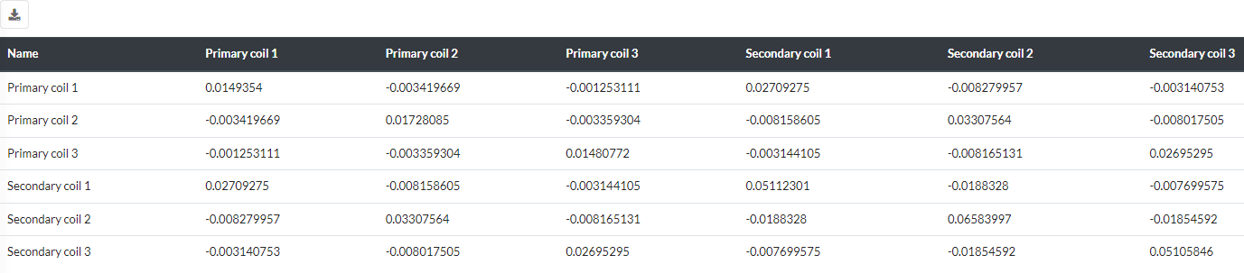
In a system comprising N coils, the inductance is represented as an NxN matrix. Here, Lii signifies self-inductance, while Lij denotes mutual inductance. To facilitate this matrix representation, it’s essential to sequentially number the coils.
Forces and Torques
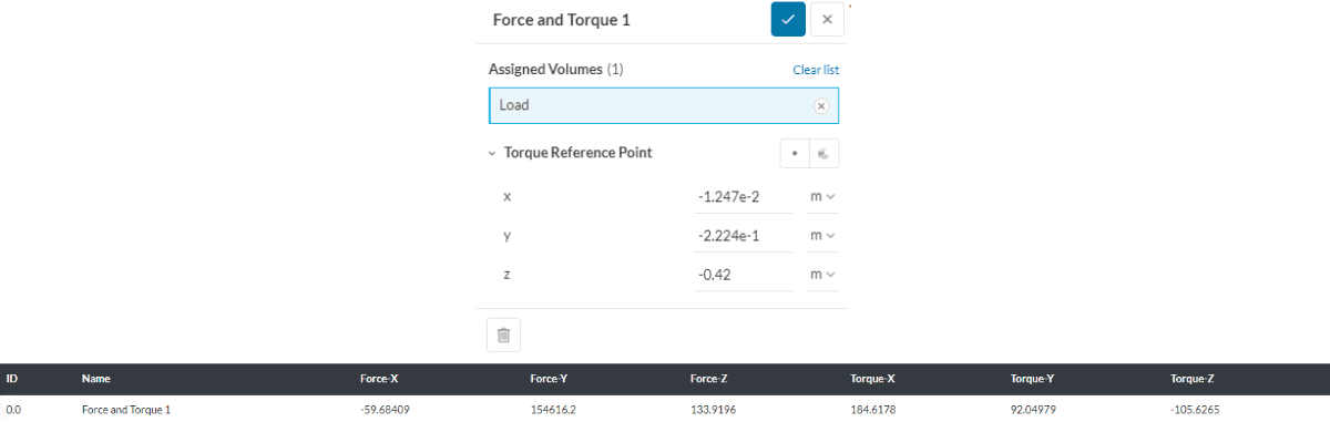
This Result control item calculates the Forces and Torques due to the electromagnetic field on a specified volume (part).
The forces and moments calculation is based on the virtual work method. This approach involves determining the change in the overall magnetic energy as the object is moved a distance \(\Delta s\) along the direction of the desired force component.
This yields that the force along the displacement direction \(s\) is:
$$ F_s = \frac{W_2 – W_1}{\delta s} $$
Where \(W\) is the virtual work and can be computed as:
$$ W = \frac{1}{2} \int{B \cdot H \, dv} $$
The torque can be obtained by rotating the component by a differential degree \(\Delta \phi\) around any of the Cartesian axes:
$$ \tau = \frac{W_2 – W_1}{\Delta \phi} $$
To define a Forces and Torques output, you can simply access it under the Result control item as shown in Figure 30. Then the user is prompted to choose a volume on which the Forces and torques would be calculated. For the Torque calculation, a Torque Reference Point needs to be defined.
Motion-coupled simulations produce time-resolved electromagnetic field results that reflect the updated geometry at each time step. The electromagnetic force and torque acting on the assigned moving bodies are computed at each time step and plotted as a function of simulation time. Use these graphs to assess dynamic load profiles and identify transient peaks or oscillations.
Useful to know about the virtual work method
In order to obtain accurate results when using the virtual work method, it is important that the body on which the forces and torques are calculated on, is surrounded by force-free materials (e.g. air). Force-free materials are substances that neither exert forces on electric charges nor interact with magnetic fields. They are typically insulators, no current flows through them, and have a magnetic permeability equal to that of free space.
Force calculation in an Electrostatic simulation
The floating potential boundary condition should not be used on a conductor if the forces on that conductor are to be computed.
Probe Points
Probe Points are user-defined, discrete spatial coordinates placed within the computational domain of an electromagnetic simulation model. They function as virtual sensors used to extract and monitor specific field quantities at precise locations inside the model.
These points provide enhanced control and precision for monitoring and analyzing simulation results.
Users define probe points by creating specific point geometry primitives and inputting the exact spatial coordinates (x, y, z) into the simulation setup. The solver then reports the value of the selected EM variables (such as field components) at these coordinates throughout the simulation run or as post-processing output.
Coils Output Table
Depending on the simulation model (e.g. Magnetostatics, Time-Harmonic Magnetics, or Time-Domain Magnetics) the coils table output provides relevant information about the coils. Such as resistances, flux linkages, induced voltages, etc.
Note that, the outputs in the coils output table for Time-Harmonic magnetics and Time-Domain magnetics represent the peak values and not RMS.
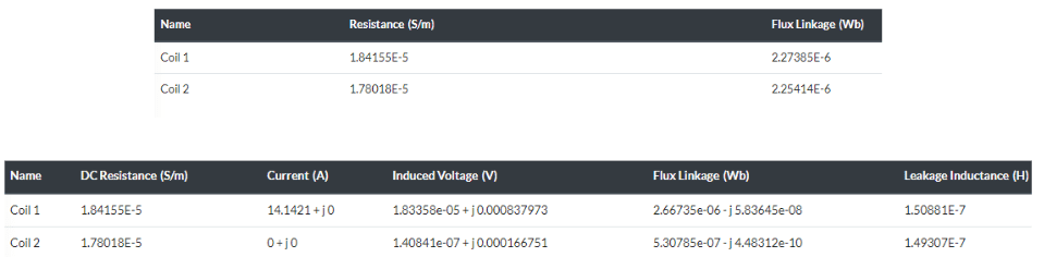
In the following, a brief description of each item from the tables in Figure 33 above is given.
Resistances/ DC Resistance
Direct current (DC) resistance refers to the opposition encountered by an electrical conductor to the flow of direct current. This resistance is a fundamental property of conductors and is governed by factors such as the material’s resistivity, cross-sectional area, and length.
Ohm’s Law, formulated by German physicist Georg Simon Ohm, states that the current \(I\) flowing through a conductor is directly proportional to the voltage \(V\) across it and inversely proportional to the resistance \(R\) of the conductor. Mathematically, this relationship is expressed as \(V = IR\).
The resistance unit is ohm (Ω). Resistance is influenced by the material from which the conductor is made. For instance, materials like copper and silver have low resistivity and are commonly used in electrical wiring due to their excellent conductivity. In contrast, materials like rubber and glass have high resistivity and are used as insulators.
Depending on the choice of coil (e.g. either a solid or stranded coil) the caluclation method can differ. For a stranded coil, the DC resistance is calculated by the formula:
$$ Resistance = \frac{4NL}{\sigma \pi d^2} $$
Where
\(N\): Number of turns,
\(L\): Length of wire,
\(\sigma\): Electrical conductivity of wire,
\(d\): Diameter of wire.
In the case of a solid coil, the resistance is calculated based on the finite element formulation to solve an electrical conduction problem which then yields the resistance value.
Flux Linkage
Flux linkage describes the relationship between magnetic flux and the number of turns in a coil or circuit. It indicates how the magnetic flux generated by one turn of the coil is linked to adjacent turns of the coil. In simple terms, it quantifies the total magnetic flux that passes through a closed loop or coil of wire.
When a magnetic field changes in strength or orientation, it induces an electromotive force (EMF) in any nearby conductors or coils, according to Faraday’s law of electromagnetic induction. The amount of induced voltage is directly proportional to the rate of change of magnetic flux linking the coil, which in turn depends on factors such as the strength and orientation of the magnetic field and the number of turns in the coil.
Mathematically, flux linkage \(\psi\) is expressed as the product of the magnetic flux \(\phi\) and the number of turns \(N\) in the coil, \(\psi = \phi * N \). The unit of flux linkage is Weber \((Wb)\).
Flux Linkage can also be calculated from the product of the inductance with the current \(\psi = LI\), which is the equation used in the simulation.
$$ \psi_i = \sum_{j=1}^\infty L_{ij} I_j $$
Where
\(\psi_{i}\) = Flux Linkage crossing coil i,
\(L_{ij}\)= Mutual Inductance between coils i and j,
\(I_j \) = Current in coil j.
Leakage Inductance
Leakage inductance is a phenomenon encountered in transformers and inductors due to imperfect coupling between their primary and secondary windings or between adjacent turns in the same winding. It describes the portion of the total inductance that does not contribute to the desired energy transfer between the primary and secondary sides but instead leaks magnetic flux.
In an ideal transformer or inductor, all of the magnetic flux generated by the primary winding would link perfectly with the secondary winding or adjacent turns, resulting in maximum energy transfer. However, in reality, there is always some degree of leakage flux that fails to link with the secondary winding or neighboring turns due to factors such as magnetic flux dispersion, geometric irregularities, and insulation between winding layers.
Leakage inductance manifests itself as an additional inductive impedance in series with the primary windings. This impedance limits the rate of change of current and voltage across the windings, affecting the device’s performance characteristics such as voltage regulation, efficiency, and transient response.
Although leakage inductance is generally considered undesirable in many transformer and inductor applications, it can also be intentionally introduced for specific purposes. For instance, in resonant transformers and inductors used in high-frequency power converters, controlled leakage inductance helps to shape the frequency response and improve circuit efficiency.
In an electromagnetic simulation on SimScale, the leakage inductance is calculated only when there are 2 coils in the simulation model:
Leakage inductance1 = \(1 – K_{12} * L_{11}\) ; Leakage inductance2 = \(1 – K_{12} * L_{22}\)
Where:
\(K_{12}\) is the coupling coefficient of coils 1 and 2,
\(L_{11}\) self-inductance of coil 1,
\(L_{11}\)self-inductance of coil 2.
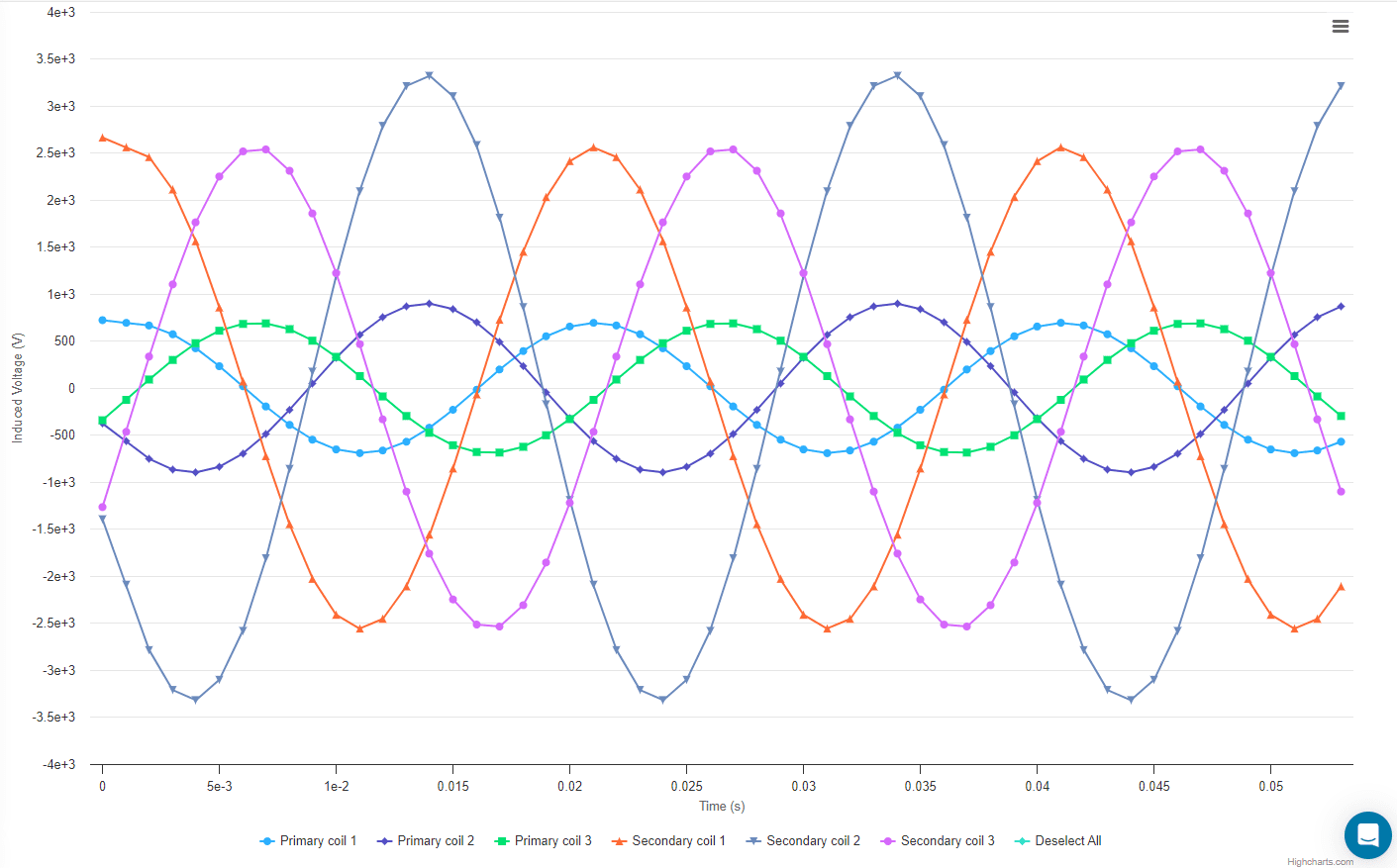
Induced Voltage
Induced voltages refer to the electromotive force generated in a conductor when subjected to a changing magnetic field, as described by Faraday’s law of electromagnetic induction.
In a Time-Harmonic magnetic simulation, the induced voltage is calculated as follows:
$$ V_i = – \frac{d\Phi_i}{dt} $$
Which in the time-harmonic formulation becomes:
$$V_i = C_j \omega \Phi_i $$
Where
\(\Phi_i\) is the flux linkage crossing coil i,
\(C_j\) is the complex j = \(\sqrt{-1}\) ,
\(\omega\) is the angular frequency.
Coupling Coefficients
Coupling coefficients represent the degree of electromagnetic coupling between two circuits or components. They quantify how effectively energy or signals are transferred from one part of a system to another. These coefficients are particularly important in understanding and designing electromagnetic systems, where interactions between components are common.
Think of coupling coefficients as a measure of how much electromagnetic influence one part of a system has on another. Electromagnetic fields generated by one circuit can induce voltages or currents in another circuit, and the coupling coefficient expresses the efficiency of this transfer.
The coupling coefficient between two coils can be calculated as follows:
$$ K_{ij} = \frac{L_{ij}}{\sqrt{L_{ii}L_{jj}}} $$
Where \(K_{ij}\) is the coupling coefficient between coils i and j,
\(L_{ij}\) is the mutual inductance of coils i and j,
\(L_{ii}\) is the self-inductance of coil i,
\(L_{jj}\) is the self-inductance of coil j.
This formula provides a quantitative measure of the extent of coupling between two components. The value of the coupling coefficient ranges between 0 and 1, where:
\(K=1\) indicates perfect coupling, meaning all the flux generated by one component is linked with the other.
\(K=0\) implies no coupling, indicating that there’s no mutual influence between the components.
It’s worth noting that this formula applies specifically to mutual inductance and self-inductances in the context of magnetic coupling.
Impedances
Impedance in electromagnetics refers to the opposition that a circuit or component offers to the flow of alternating current (AC). It’s a measure of how much a device resists the flow of alternating current, just as resistance measures the opposition to the flow of direct current (DC).
Impedance combines both resistance and reactance. Resistance is the opposition to the flow of current due to the material properties of the conductor. Reactance, on the other hand, arises due to the effects of inductance and capacitance in a circuit. Inductance opposes changes in current, while capacitance opposes changes in voltage. Together, resistance, inductance, and capacitance define the impedance of a circuit. In AC circuits, impedance can vary with frequency due to the frequency-dependent behavior of inductors and capacitors.
Think of impedance as a measure of how “stubborn” a circuit is when an alternating current tries to flow through it.
In a Time-Harmonic Magnetic analysis, the inductance and resistance of a coil deviate from DC values due to skin and proximity effects. These effects are accurately taken into account to compute the resistance and inductance matrices that encompass the self and mutual terms. Subsequently, the impedance matrix is derived from these matrices.
Impedance can be represented as a complex number, where the real part represents resistance and the imaginary part represents reactance. The unit of impedance is the Ohm \(\Omega\).
The formula for calculating impedance is:
$$ Z_{ij} = R_{i} + C_{j} \omega L_{ij} $$
Where,
\(Z_{ij}\) is the impedance of coil i and j,
\(R_i\) resistance of coil i,
\(C_j\) is the complex j = \(\sqrt{-1}\),
\(L_{ij}\) is the inductance of coils i and j.
Inductive and capacitive reactance
Capacitive reactance is not taken into account in a Time-Harmonic Magnetic simulation, since one of the assumptions behind the time-harmonic model implies that the model should not store any relevant electrical energy, i.e. it does not contain any relevant capacitance.
Resistance table output in a Time-Harmonic Magnetic Simulation
The additional resistance table output in a Time-Harmonic Magnetic simulation is simply all the real terms from the impedance table.
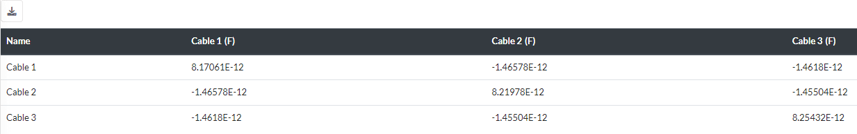
Capacitances
Capacitance measures how much electric charge is stored between conductors at a given electric potential. It’s there whenever you have two insulated conductors nearby. Typically, it’s calculated as the total electric charge on an object divided by its potential. In MKS units, capacitance is measured in farads \(F\). One farad means one volt of potential for one coulomb of charge. However, most capacitors in electronics are way smaller, often measured in Microfarads \(\mu F\), Nanofarads \(nF\), or Picofarads \(pF\).
For a system with \(N\) conductors, capacitance is represented by an \(N \times N\) matrix. Within this matrix, \(C_{ii}\) stands for self-capacitance, while \(C_{ij}\) denotes mutual capacitance. Self-capacitance means the charge needed to increase the potential of a single conductor by one volt. Mutual capacitance is the capacitance between two conductors when the influence of all other conductors is excluded.
To enable capacitance calculation in the simulation, click on the ‘Result control’ item, and then a pop-up window will appear on the top right of the simulation tree similar to what is shown in Figure 30 for the inductance matrix in a magnetostatic simulation.
Capacitance Calculation
In order to calculate the capacitance matrix: Assign a floating potential to each conductor in the system and a fixed zero voltage to conductors that are meant to be grounded.
Results and Post-Processing
Motion-coupled simulations produce time-resolved electromagnetic field results that reflect the updated geometry at each time step. In addition to standard field outputs (magnetic flux density, field intensity, etc.), the following quantitative results are available:
Force and Torque vs. Time
The electromagnetic force and torque acting on the assigned moving bodies are computed at each time step and plotted as a function of simulation time. Use these graphs to assess dynamic load profiles and identify transient peaks or oscillations.
Torque vs. Rotor Angle
For rotational motion, torque can also be visualized as a function of rotor angular position. This is particularly useful for characterizing torque ripple and evaluating motor performance across a full electrical cycle.
Field Animation
Electromagnetic field results (such as magnetic flux density) can be animated across time steps, showing how the field evolves as the moving component advances along its motion path. The mesh is updated in the visualization to reflect the physical position of moving parts at each time step.
Numerics
Numerical settings play an important role in the simulation configuration. They define how to solve the equations by applying proper discretization schemes and solvers to the equations. They help enhance the stability and robustness of the simulation.
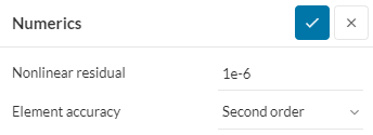
Element Accuracy
The Element accuracy setting allows the user to choose the order of the finite element, a selection between first-order (linear shape functions) and second-order (parabolic shape functions) is available.
The default Element accuracy is second order. It is recommended to leave it as such when higher accuracy is desired, especially when calculating forces and torques. The second-order element, while more accurate, does come with higher computational demands compared to the first-order element due to the additional degrees of freedom in the elements.
Nonlinear Residual
This represents the maximum permissible error in the iterative solver. When dealing with a well-defined model, the iterative solver will continue its iterations until it achieves an error lower than this specified value. Should it be unable to attain an error smaller than this threshold, it will terminate and report a failure. The smaller the nonlinear residual value the tighter the convergence of the simulation will be, which can result in a more accurate solution at the expense of an additional solving time.
Simulation Control
The Simulation control settings define the general controls over the simulation. Such as choosing the number of processors for the simulation job, here one can choose between 1-192 cores, or to leave the selection as automatic, and SimScale attempts to choose the best suited machine for the job at hand.
Moreover, Users can define the Maximum runtime of the simulation here which dictates the maximum runtime of your simulation in real-time. The simulation run stops when it goes beyond this value.
In a transient simulation, the user can define the simulation End time and the time increment needed to resolve the field phenomena of interest.
The Core loss reference period defines the time window over which magnetic core losses (hysteresis, eddy current, and excess losses) are evaluated and averaged. In practice, it is usually set to the duration of one complete cycle of the excitation waveform, such as a single period of an applied AC voltage or current.
The Time-periodic acceleration feature can be enabled to speed up convergence toward the periodic steady-state response of the system when it is excited by a time-periodic source, such as sinusoidal or PWM waveforms. Instead of simulating multiple cycles for the solution to naturally settle, the solver intelligently predicts and accelerates the evolution of the magnetic field by leveraging the known periodicity of the system. This significantly reduces computation time while still capturing the essential steady-state behavior, making it especially useful for analyzing losses, torque ripple, and harmonic content in electric machines and transformers.

Mesh
Meshing is the process of discretization of the simulation domain. That means we split up a large domain into multiple smaller domains and solve equations for them.
For an electromagnetic analysis, the standard algorithm is available. For more information about meshes, make sure to check the dedicated page.
Related Documentation
References
- https://www.flukenetworks.com/blog/cabling-chronicles/101-series-stranded-vs-solid-patch-cords
- https://www.nde-ed.org/Physics/Magnetism/Demagnetization.xhtml
Last updated: June 4th, 2026
Did this article solve your issue?
How can we do better?
We appreciate and value your feedback.


