CFD Numerics: Numerical Schemes

Numerical schemes calculate the values for different terms like derivatives, e.g. gradient and interpolations of values from cell centers to nodes. A wide range of numerical schemes are available that provide flexibility and freedom. 

Keyword	Category of mathematical terms
interpolation schemes	point-to-point interpolations of values
surface normal gradient schemes	component of gradient normal to a cell face
gradient schemes	gradient \(∇\)
divergence schemes	divergence \(∇ ∙\)
Laplacian schemes	Laplacian \(∇^2\)
time differentiation schemes	first and second-time derivatives \(∂ \over\ ∂t\) ,\(∂^2 \over\ ∂^2t\)

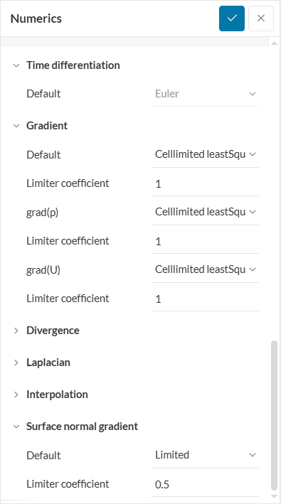
Time Differentiation

The time differentiation schemes calculate the rate of change of the variables over time. When selecting a time scheme it must be noted that a problem designed for transient analysis will not necessarily run with steady-state and visa-versa.

The table below shows all the possible types. Some may or may not be available depending upon analysis type.

Scheme	Description
Euler	first-order, bounded, implicit
local Euler	local time step, first order, bounded, implicit
Crank Nicholson \(ψ\)	second-order, bounded, implicit
backward	second-order, implicit
steady state	does not solve for time derivatives

The first order bounded, ‘Euler’ is the most robust while the second-order ones are more accurate. Backward is a second-order time-differentiation scheme that gives higher accuracy but may reduce stability.

Interpolation Scheme

The interpolation schemes define the terms that are interpolated values from cell centers to face centers. These are primarily used in the calculation of velocity to the face centers for the calculation of flux. There are numerous interpolation schemes but the default scheme in all the cases is the ‘Linear interpolation’ i.e a 2nd order interpolation scheme.

Gradient Schemes

The grad Schemes interpolate the values for the gradient terms in the differential equations. The discretization scheme available are listed as follows:

Discretization scheme	Description
Gauss <interpolationScheme>	second-order, Gaussian integration
least squares	second-order, least squares
fourth gradient	fourth-order, least squares
celllimited <gradScheme>	cell limited version of one of the above schemes

‘Gauss’ represents the standard finite volume discretization using the Gaussian integration that requires the interpolation from cell centers to face centers. The recommended types are the second-order accurate ‘Gauss Linear’ or ‘Least squares’ schemes. 

For better stability and robustness, the ‘cellLimited’ versions of both can be used. The ‘Limiter coefficient’ of 1.0 means full boundedness/limiting of values while 0 means no limiting.

Divergence

The divergence schemes are used to calculate the convection term in the fluid dynamics differential equations \(∇ ∙(ρUU)\) :

Scheme	Numerical behavior
linear	second-order, unbounded
skew linear	second-order, (more) unbounded, skewness correction
cubic corrected	fourth-order, unbounded
upwind	first-order, bounded
linear upwind	first/second-order, bounded

• Gauss upwind: first-order bounded, generally robust but compromises accuracy
• Gauss linear: second-order, unbounded. Accurate but not robust
• Gauss linear upwind: second-order, upwind-biased, unbounded, that requires discretization of the velocity gradient to be specified.
• Gauss limited linear: a linear scheme that limits towards upwind in regions of rapidly changing gradient; requires a coefficient, where 1 is the strongest limiting, and shifting towards linear as the coefficient tends to 0.
• Gauss linear upwind v \(∇u\): second-order, upwind, bounded, is a good choice for stable second-order linear scheme.

Surface-normal Gradient

A surface normal gradient is calculated at a cell face and is defined as the component normal to the face, of the gradient of values at the centers of the 2 cells.

Scheme	Description
corrected	explicit non-orthogonal correction
uncorrected	no non-orthogonal correction
limited \(ψ\)	limited non-orthogonal correction
bounded	bounded correction for positive scalars

For maintaining accuracy, an explicit non-orthogonal correction can be added to the orthogonal component, known as the corrected scheme. The correction increases in size as the non-orthogonality increases.
Beyond 70°, the explicit correction can be so large that it can cause a solution to become unstable. The solution can be then stabilized by applying the limited scheme which requires a coefficient \(ψ\), 0 ≤ \(ψ\) ≤  1, where:

• \(ψ\) = 0 : corresponds to uncorrected,
• \(ψ\) = 0.333 : non-orthogonal correction ≤ 0.5 \( \times\) orthogonal part,
• \(ψ\) = 0.5 : non-orthogonal correction ≤ orthogonal part,
• \(ψ\) = 1 : corresponds to corrected.

Usually, \(ψ\) is chosen to be 0.33 or 0.5, where:

• 0.33 offers greater stability,
• 0.5 greater accuracy.

Laplacian

The typical Laplacian term is \(∇ ∙(ν∇U)\), which is the diffusion term in the momentum equations, that is calculated by the laplacianSchemes. Only the Gauss scheme is available for discretization and further requires a selection of both an interpolation scheme for the diffusion coefficient and a surface normal gradient scheme:

Gauss <interpolationScheme> <snGradScheme>

Scheme	Category of mathematical terms
corrected	unbounded, second-order, conservative
uncorrected	bounded, first order, non-conservative
limited \(ψ\)	blend of corrected and uncorrected
bounded	first-order for bounded scalars

• Gauss linear corrected: is a 2nd order accurate with corrected gradients.
• Gauss linear limited corrected 0.5: 2nd order, corrected, with limiter value 0.5

Last updated: January 21st, 2022