Physical Contacts

Physical (or “nonlinear”) contacts enable you to calculate realistic contact interaction between two parts of the assembly. Also, it allows calculating the self-contact between different faces of the same part. Unlike linear contacts, those faces are not just connected via linear relations but the actual contact forces are computed.

To enable a nonlinear interaction, you have to define contact pairs of faces or face sets. For those faces the distance between each other is tested during the simulation, and, in the case that a face pair gets in contact, the interaction forces are taken into account, preventing those faces from interpenetrating each other. As those forces only occur in the case of contact the interaction is a nonlinear phenomenon and thus only applies for nonlinear analyses.

The Physical contacts settings panel offers the following choices:

The physical contact solution algorithm works by performing two independent steps:

1. Compute the non-linear deformation of the geometry (Nonlinearity Resolution): The deformation of the geometry due to the boundary conditions is computed at the beginning of each time step, without taking into account the physical contact condition.
2. Compute the contact compliance condition (Contact Nonlinearity Resolution): The interpenetration between contact pairs is computed, and the geometry is updated accordingly to enforce the physical contact condition. Then, the contact pressure is computed and the forces are registered for the next time step.

The following general parameters are available for the global physical contact algorithm:

• Nonlinearity resolution: Selects the algorithm used to compute the nonlinear deformation of the geometry before the contact resolution (first step of the algorithm above). The available choices and specific parameters are:
  • Fixed point: An external iteration loop is added on top of the newton iterations to solve the nonlinear deformation. The available parameters for this algorithm are:
    • Geometry update: Indicates mode of operation of the algorithm between Automatic, Manual, or No update.
    • Max num iterations: Available in the Automatic mode, it indicates the maximum number of iterations of the algorithm. If this criterion is reached, a divergence of the computation is reported.
    • Iteration Criterion: Available in the Automatic mode, it indicates the threshold of the algorithm to consider that convergence has been achieved.
    • Number of iterations: Available in the Manual mode, it indicates the fixed number of iterations to be performed.
  • Newton: The geometry resolution is included in the global newton iterations. The only available parameter is the Iteration criterion, which is the threshold of the contact penetration residual to be considered when the solution is converged.
• Friction: Allows to select if the tangential friction force of type Coulomb will be considered in the simulation. If selected, there are two available choices for the algorithm: Newton and Fixed-point automatic, with the same parameters as described above. This allows the solution of the friction force to use a different algorithm than the normal force.
• Contact nonlinearity resolution: Selects the algorithm used to compute the contact compliance deformation. The available choices are:
  • Newton: The geometry update is included in the global newton iterations.
  • Fixed Point: An external iteration loop is added on top of the global newton iterations to solve the geometry. The iterations number control has two variations:
    • Maximum number: When the Max num iterations are reached, a divergence error is reported.
    • Multiple of slave nodes: The maximum number of iterations is the number of nodes in the slave surface times the Multiple value.
• Contact smoothing: Smoothing of the mesh surface normals. It is useful in the case of curved surfaces, especially with coarse meshes.
• Enable heat transfer: Allow heat transfer between master and slave faces. This option considers the faces to be in perfect thermal contact, even if they are not mechanically in contact.

Contact Pairs Definition

For each contact pair definition, click on ‘+’ next to Physical contacts and the following parameters are available:

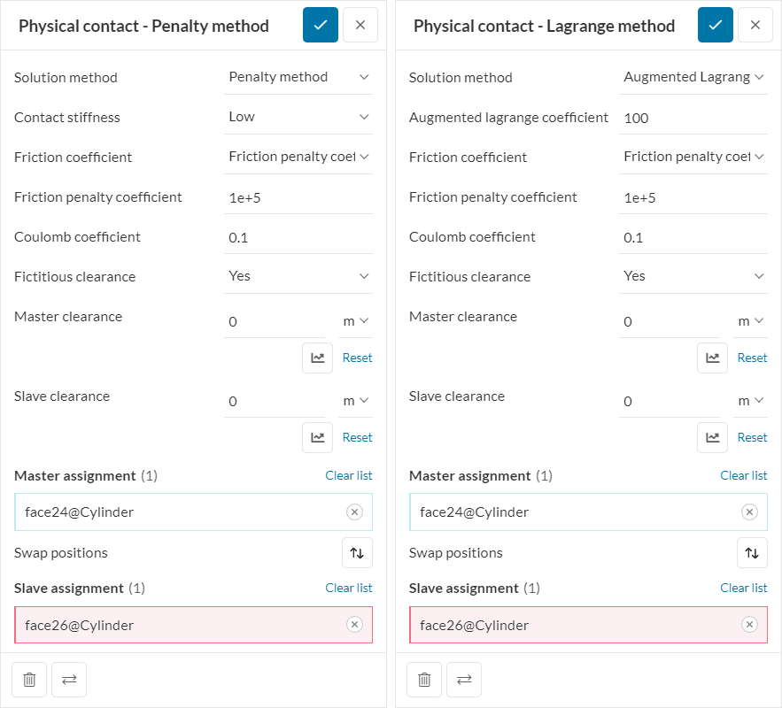
• Solution Method: For each physical contact definition, it is possible to choose the model between the Penalty method and the Augmented Lagrange method (explained below). The following parameters control the solution:
  • Penalty Coefficient: Available for the penalty method, it is the constant for the contact pair that determines the ‘stiffness’ for the contact penalty.
  • Augmented Lagrange Coefficient: Available for the Lagrange method, it is the value of the Lagrange multipliers for the augmented contact equations.

To learn more about this physical contact setting and prediction of the coefficients, please check this article.

• Friction Coefficient: Allows to choose the friction solution method for the contact pair, with the same choices as for the normal force resolution.
  • Friction penalty coefficient: Penalty coefficient for the friction force resolution.
  • Friction augmentation Lagrange coefficient: Lagrange multiplier for the friction force resolution.
• Coulomb coefficient: Ratio between the normal and the tangential friction forces.
• Fictitious clearance: This allows the introduction of an artificial separation gap between the contact. surfaces. If enabled, the contact is considered to be active when the gap is smaller than the sum of Master clearance and Slave clearance. The clearance can be input as a variable value. The table below contains of examples in order to provide a better idea of how the Fictitious Clearance values affect the state of contact between the two surfaces.
• Master and slave assignment: Specifying master-slave assignments have a significant impact on solver performance. Please check this article to learn about the three basic rules.

Case	Initial State	Fictitious Clearance	Final State
1	2 \(mm\) GAP	1 \(mm\)	2 \(mm\) GAP (no contact active)
2	2 \(mm\) GAP	-1 \(mm\)	2 \(mm\) GAP (no contact active)
3	2 \(mm\) GAP	3 \(mm\)	3 \(mm\) GAP (contact active)
4	2 \(mm\) OVERLAP	1 \(mm\)	1 \(mm\) GAP (contact active)
5	2 \(mm\) OVERLAP	-1 \(mm\)	1 \(mm\) OVERLAP (contact active)
6	2 \(mm\) OVERLAP	3 \(mm\)	2 \(mm\) OVERLAP (contact inactive)

Penalty Contacts

In a penalty contact solution method the contact interaction between the bodies is handled via spring elements that model the stiffness of the contact. Hence, in a penalty approach, the faces in contact may penetrate each other slightly depending on the defined contact stiffness that couples the interpenetration with the consequential reaction forces.

It is called the Penalty method because the interpenetration creates forces that act to prevent further intersection, penalizing this behavior.

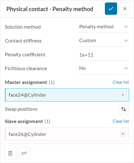
The Contact stiffness is defined by the coefficient of the linear penetration model. The higher the penalty coefficient, the stiffer the contact gets, which is desired in most cases, as bodies usually are not intended to penetrate at all.

There are four options for contact stiffness: low, moderate, high, and custom. The larger the contact stiffness, the less interpenetration is observed. However, convergence becomes increasingly more difficult for larger penalty coefficients. A trade-off between realistic behavior and optimization for convergence needs to be found.

When using a low contact stiffness, the penalty coefficient receives a value 50 times larger than the Young’s Modulus of the softest material that takes part in a given contact. With a moderate and high contact stiffness, the penalty coefficient receives a value 200 and 1000 times larger than the Young’s Modulus of the softest material, respectively.

With a custom contact stiffness, the user can choose any value for the penalty coefficient.

Lagrangian Contacts

In the Augmented Lagrange contact solution method the contact interaction between the bodies is handled via additional Lagrange equations that account for the contact conditions. As opposed to the penalty method, the contact equations are solved exactly and thus no penetration between the contact faces may occur.

Contact Monitoring

During nonlinear simulations including physical contacts, you are provided with contact monitoring plots which will keep you in the loop on contact penetration and solution convergence, giving you confidence and control over your result outputs.

The following plots will be available under the simulation run, and will be updated as the computation advances:

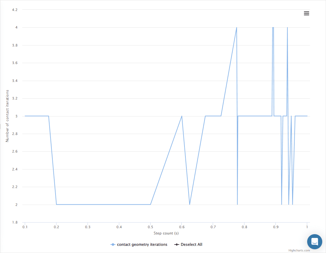
Number of Contact Iterations

This plot presents the number of fixed point iterations that were performed for convergence to be achieved at each load or time step.

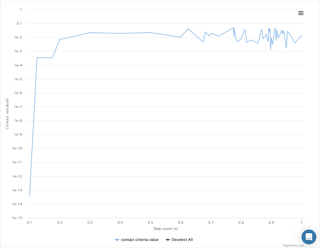
Contact Residuals

This plot presents the contact residual at the last fixed point iteration of each time or load step when convergence is considered to be achieved according to the iteration criterion.

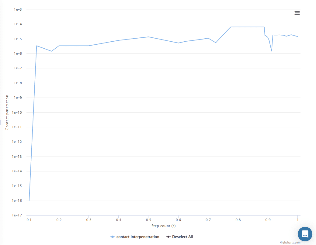
Contact Penetration

This plot presents the sum of all penetrations in physical contact pairs, each one measured as the distance between a node in the slave surface and the master surface, in units of length, when the node enters the volume of the master surface.

Last updated: June 24th, 2024