Integrated Post-Processor
The online post-processor integrated into SimScale is compatible with all your old/new projects and simulations that you create.
This document provides a detailed overview of SimScale’s post-processor. It can be used as a general source of information and also as a follow-along. For easy understanding, an example of a fluid flow through a pipe is used to relate the features to an actual simulation.
If you would like to follow along or play with the various filter settings, make sure to open the sample project below:
Post-Processing
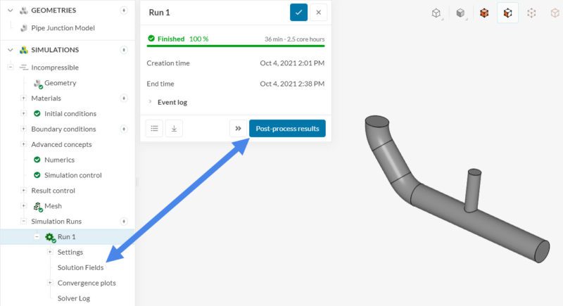
Firstly, when a simulation is successful or has results available, the run dialog box will prompt a ‘Post-process results’ button. Clicking this button or selecting ‘Solution Fields’ in the simulation tree will open the results in the online post-processor.
Note
The result will only load when you stay in the same tab where the Workbench is opened. The load time for the results will depend on the size of the data. The larger the data, the longer it takes to load results.
Overview
The post-processing environment contains several functions and filters that allow you to obtain a visual representation of the results. The figure below contains an outline of the post-processor:
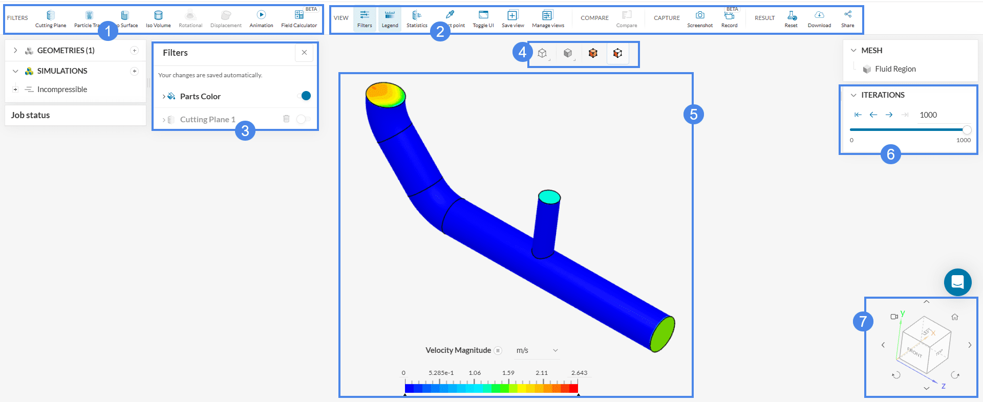
- Filters creation toolbox: Many filters, such as Cutting plane and Particle trace, are available in the post-processing environment. They are useful to obtain more insights into your results.
- Additional tools: To the right of the filters toolbox, you will find useful tools, such as Screenshot and Inspect point, amongst others. An on/off toggle for the legend is also available.
- After creating a filter, it will be listed in the Filters box. The filters box allows you to configure each filter, as well as duplicate filters’ settings, and delete existing filters.
- Visualization and selection modes toolbox: Here you can change (from left to right) the view and render mode of the geometry, as well as choose the selection mode between Select volume and Select face.
- Viewer: This is where you can see results. A series of quick selection tools are accessible by right-clicking on the viewer.
- Frame selection toolbox: This part of the post-processor is especially useful in transient simulations. It allows you to navigate through the various result sets that were saved during the simulation run.
- The Orientation cube on the bottom-right is helpful to position the camera angle. The home icon adjusts and zoom-fits the model to the screen.
Important
Users should note the following about the Filters panel box:
Post- Processing Tools
Legend
On the top bar of the post-processor, you can choose to show or hide the Legend, as shown below:
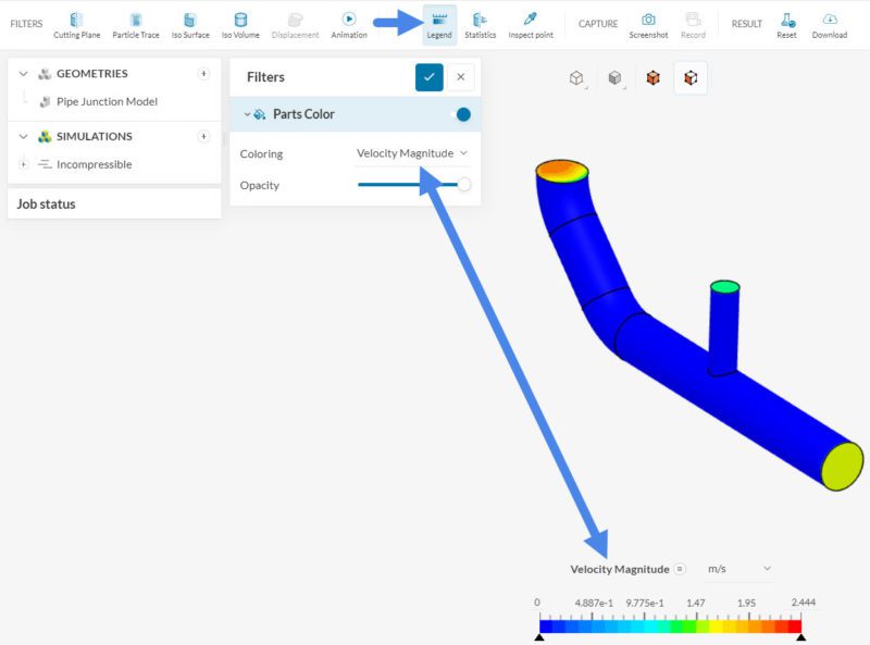
The post-processor goes through the list of filters, checking which parameters are being analyzed. Only the legend for these parameters will be visible. For example, in the image above the only parameter in the filters is velocity magnitude. Changing the field on the filters will change the legend as well.
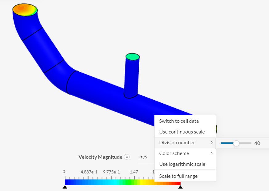
The scale bar is highly customizable, including the displayed range, units, and the number of divisions. Figure 4 shows the details:
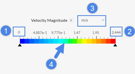
- By clicking on the minimum value of the scale range, you can set your custom values.
- Likewise, the maximum value of the range can also be changed.
- In the drop-down menu, next to the parameter’s name, you can change the units displayed on the scale.
- By right-clicking on the scale, you can change the color schemes, number of scale divisions, scale back to the full range, or even use a continuous scale.
The number of scale divisions is 20 by default. To change the number of scale divisions, right-click on the scale and adjust the Division number accordingly.
Did you know?
When you manually change the minimum and maximum values of the legend, the new range will be persistent. This means that if you run animations, step through different saved iterations or timesteps, create new filters, hide or show parts, and even exit and re-enter the post-processor, the minimum and maximum values that were manually defined will still apply.
To scale back to full range, you can right-click on the legend and select ‘Scale to full range’, as illustrated in the figure above.
Statistics and Inspect Point
The Inspect point feature is useful to obtain an accurate read on a specific point of the surface. For example, to inspect the velocity magnitude on the top inlet:
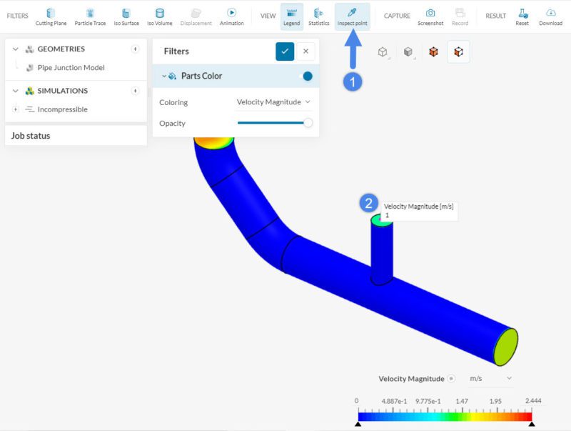
- Enable the Inspect point toggle on the top ribbon.
- Click on any point within the top inlet face. In this case, the inlet is defined by a boundary condition, so the velocity is fixed at 1 \(m/s\).
Another very useful option is Statistics. When this option is on, you can obtain detailed information about faces, volumes, and cross-sections (when used alongside cutting planes).
For example, using the Statistics feature, we can easily obtain an average for the velocity magnitude on the outlet. Figure 7 shows the steps:
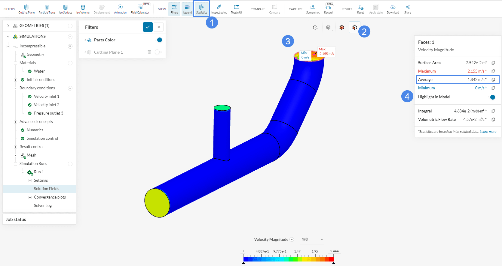
- Ensure that Statistics is toggled on
- Enable the Select face option. Note that, if your Inspect point toggle is still on, you will need to disable it to select a face.
- Click on the outlet face to select it. An information box will appear in the viewer, containing minimum and maximum values, averages, integrals, and additional information related to the selected parameter.
- Turn on ‘Highlight in Model’, which marks the points of the maximum and minimum value.
Note that the information displayed by the statistics filter is dynamic. You can select various faces and also change the parameter that is being analyzed. To make the information box disappear, you can toggle Statistics off.
Visualization and Selection Modes
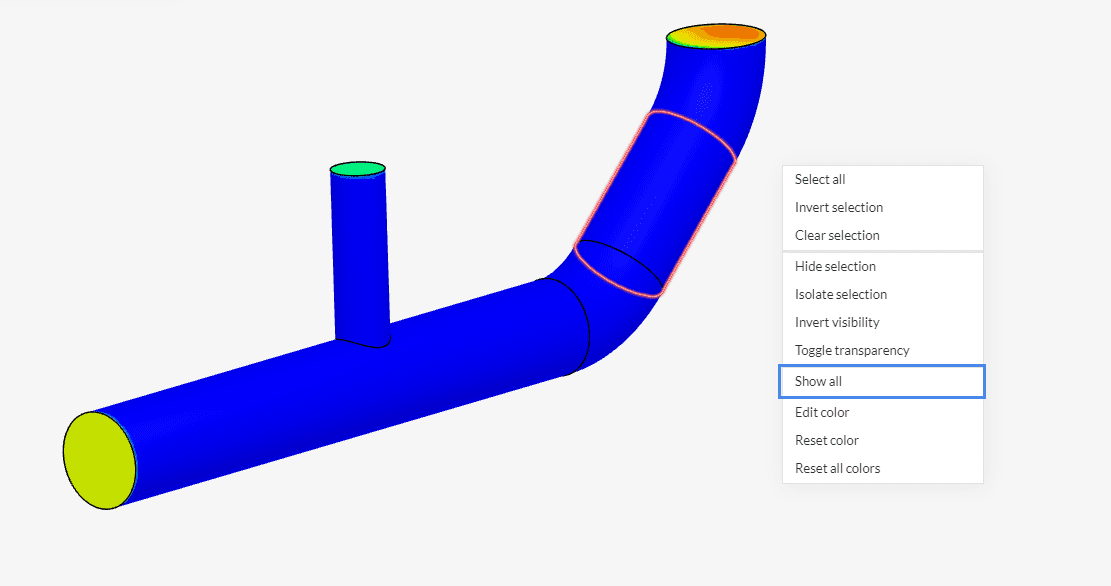
The selection modes are designed to quickly select and modify the visualization of the geometry. By right-clicking on the viewer, you will have access to many quick selection options. Some visualization options, such as Hide selection, are also available to hide the selected parts.
Hide selection is especially useful whenever we have an enclosure around the regions of interest (in external aerodynamic simulations, for instance). To make the parts visible again, right-click on the viewer, and select ‘Show all’:
Custom Coloring
SimScale allows you to set custom colors for individual surfaces or volumes, replacing the coloring of the active field function. This can help to better visualize results or generate images for presentations and marketing purposes.
Depending on the active selection mode, single or multiple faces or volumes can be colored. After the selection of faces or volumes, right-click in the viewer to open the selection panel. At the end of the options list, the following color features are listed:
- Edit Color: Set a custom color to the selected face or volume.
- Reset Color: Reset the custom color of the selected face or volume.
- Reset All: Reset all custom colors of faces or volumes.

Selecting ‘Edit Color’ will open the following options for adjusting color.

- Choose a custom color within the color field and adjust the color and transparency using the sliders.
- Enter a Hex-Cod or input, Red, Green, Blue, and Alpha values.
- Choose a color from predefined colors.
Did you know?
All colors can be created by combining Red, Green, and Blue. Monitors use an array of small red green and blue LEDs. Each LED is controlled via a byte, which can have a value from 0-255. Therefore, by setting the value for red, green, and blue, the brightness of each LED is set, which creates the desired color.
Cutting Plane
If you would like to follow along or play with the various filter settings, make sure to open the sample project below:
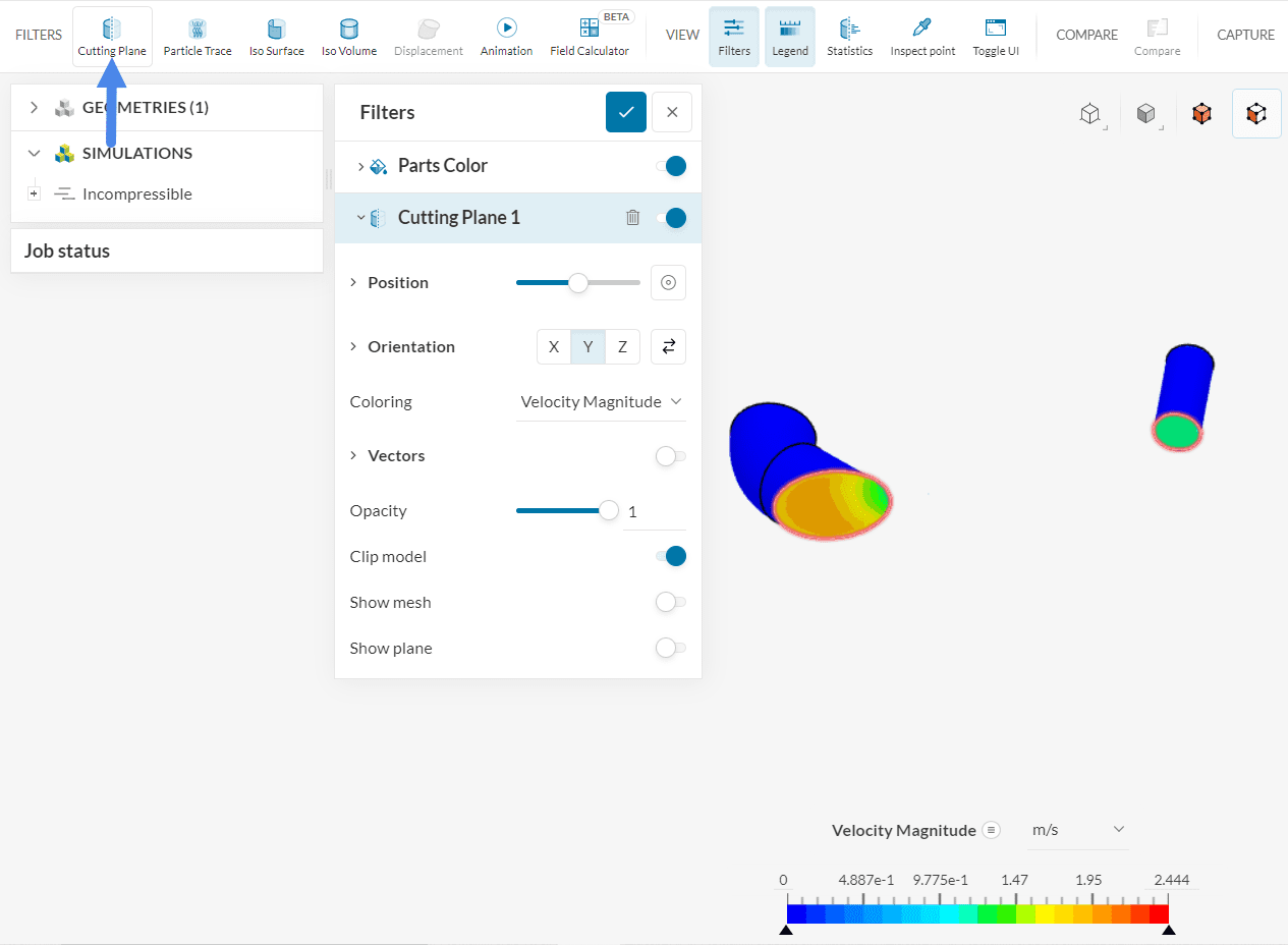
With a Cutting plane filter, you can slice the domain and visualize parameters of interest on the plane. Additional options, such as plotting velocity vectors, are also available.
To create a new filter, select the option of interest in the filters toolbox:
It is possible to use cutting planes in combination with the Statistics tool. When enabled, statistics will show average, minimum, and maximum results on the entire cutting plane and each sub-region. For example, in the image above the cutting plane generates 2 sub-regions when splitting the domain. After enabling statistics, we see the following:
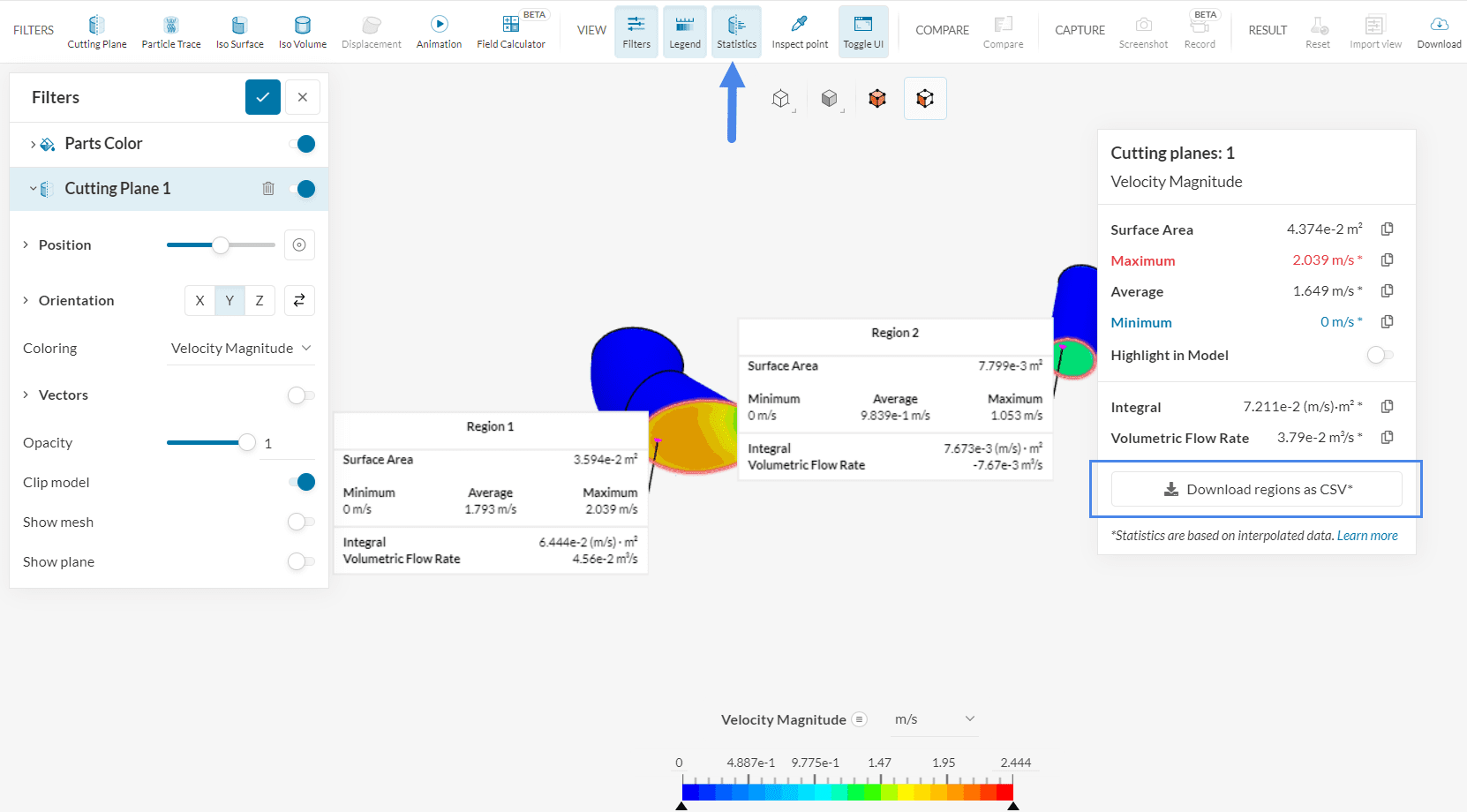
As shown above, you can download the data from each of the sub regions as a .csv file, which contains numerical data and the coordinate of the center point of each sub region. This feature is especially useful when comparing results between multiple channels in parallel. To make the statistics boxes disappear, simply disable Statistics.
Cutting planes are highly customizable. For instance, you can define an Orientation/Position, Opacity, plot Vectors, choose a Coloring option for the cutting plane, among other options.
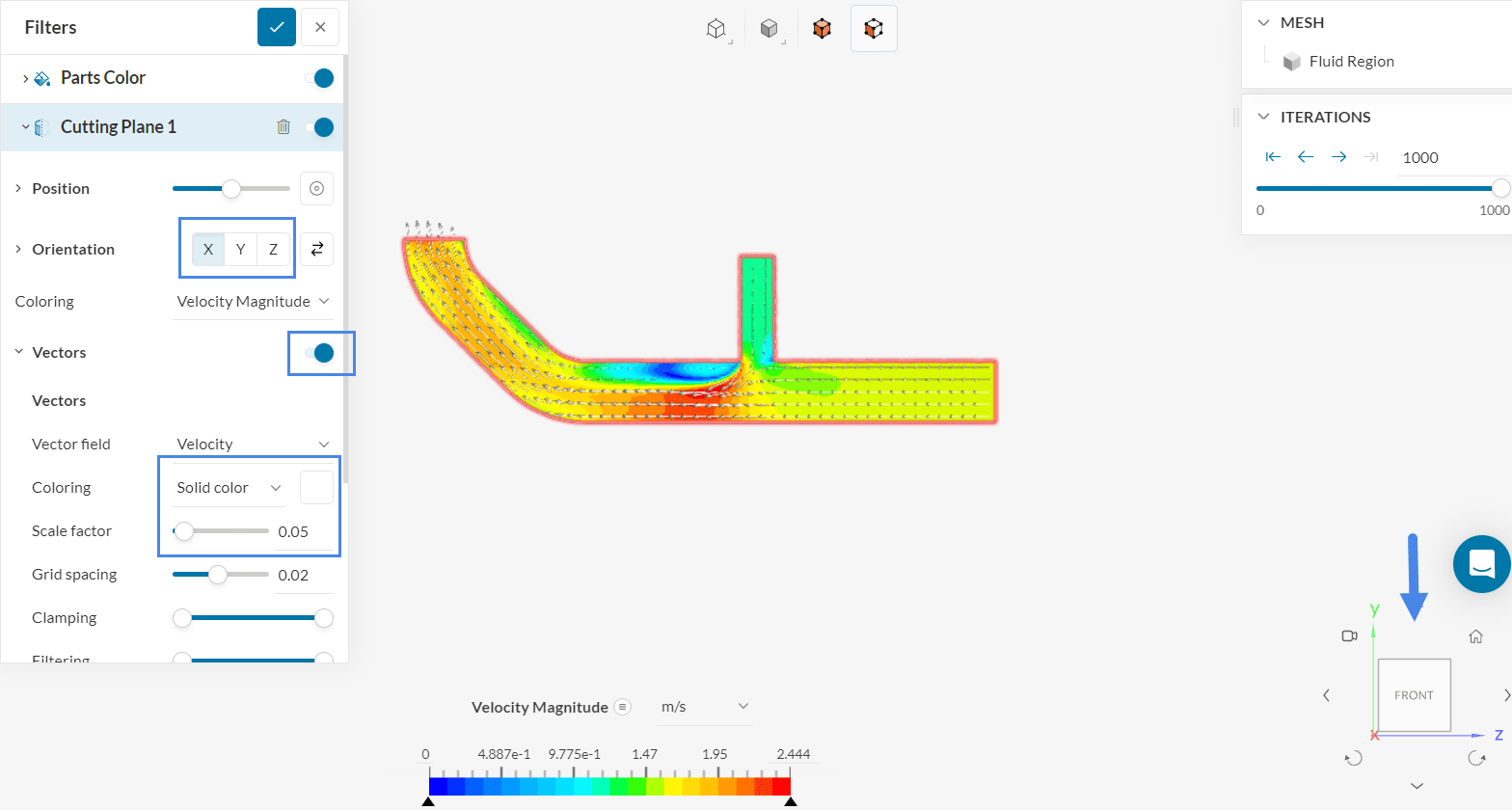
By adjusting the position and orientation of the cutting plane, taking the orientation cube as a reference, it is possible to obtain valuable insights. To add Vectors to the cutting plane, one can do as follows:
Did you know?
Within the filters panel, you will find a series of options, as in Figure 14:
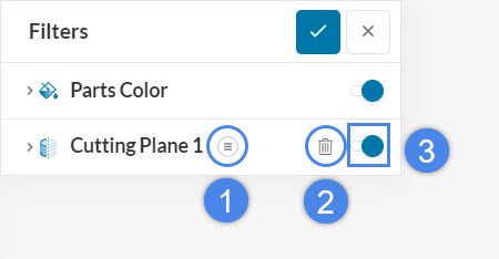
Figure 14: Options like duplicating a filter or hiding or deleting it are possible.
1. By clicking on the icon just right of the filter’s name, you can duplicate it.
2. The dustbin icon deletes a filter.
3. The ON/OFF toggle enables you to show or hide a filter.
Iso Surface and Iso Volume
The Iso surface filter is useful to show cells that match a given variable value. For example, to see where the velocity magnitude is exactly 1 \(m/s\) an Iso surface filter, with the following configuration can be created:
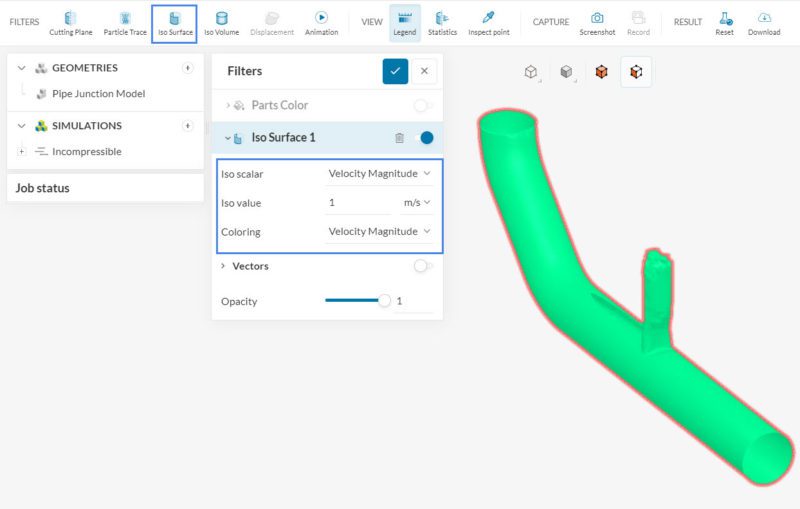
Within Iso scalar and Iso value, the user decides the criteria for highlighting the cells. With Coloring, you can choose a parameter color for the cells that satisfy the criteria.
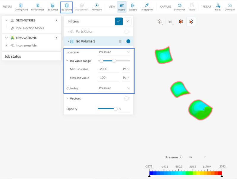
The Iso volume filter works the same way. However, instead of defining a single Iso value, the user defines an Iso value range to highlight the cells.
For example, to highlight the regions with gauge pressure levels between -2000 and -100 \(Pa\) one should proceed as follows:
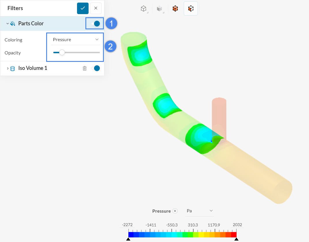
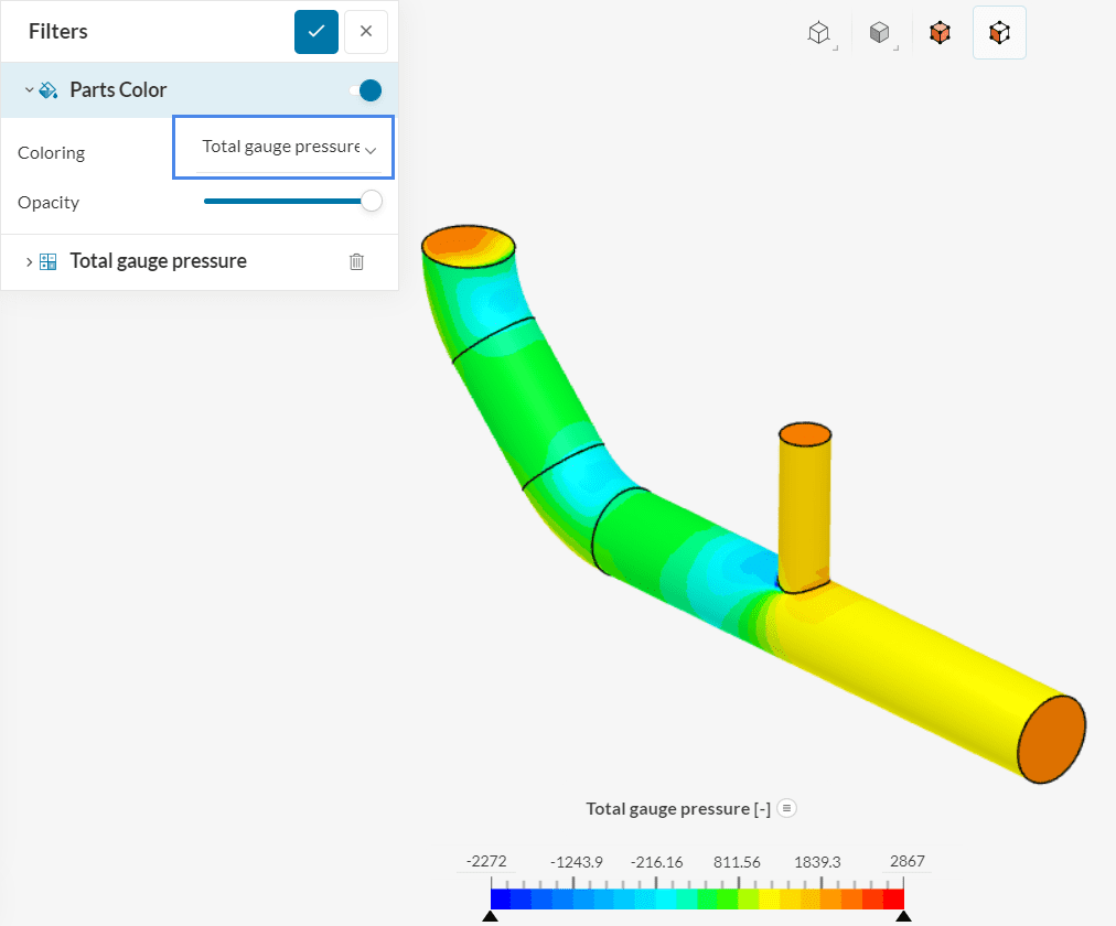
To have a clearer view of where the highlighted regions are, it’s possible to enable Parts Color with transparency. The image below shows the details:
Particle Trace
A Particle trace filter generates streamlines from a seed face. They can be useful to observe recirculation spots and flow patterns, allowing us to improve the designs.
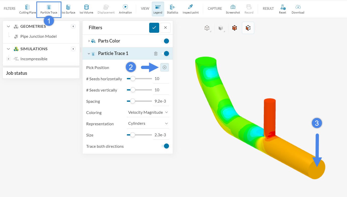
Configuring a particle trace is very simple. After creating the filter, the user needs to select a seed face, from where the streamlines are generated. Oftentimes, the inlets and outlets are good candidates for seed face. The unit of positioning as well as spacing values is meter (metric) or inch (imperial), depending on the selected unit system when creating a new project. With Pick Position enabled, you will be able to select one of the inlets as a seed face, as in Figure 18:
It is possible to duplicate the first particle trace filter, and set a second trace from the top inlet:
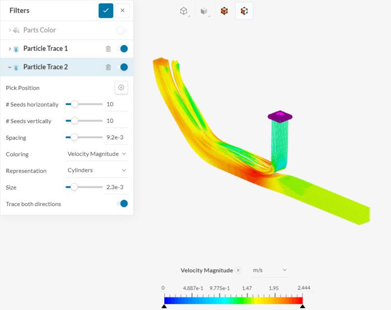
Did you know?
The Particle Trace filter is highly customizable, allowing the configuration of the following settings:
- The number of seeds, in the horizontal and vertical directions
- Spacing between two streamlines within the seed face
- Any of the parameters can be selected for the coloring of the traces. Alternatively, one can also choose to use a solid color
- For the visual representation of the traces, the user can choose Cylinders, Comets, or Spheres
- The size of the streamlines can be adjusted
- With Trace both directions, the streamlines are generated both upstream and downstream of the seed face
- Depending on the representation of the traces, more setup options may appear. The Num pulses configuration is available for spheres and comets and represents the number of particle sets in the domain at a given time.
- For comets, it is also possible to define the relative comet length. This way, each comet leaves a trail relative to its velocity, as seen in the figure below.
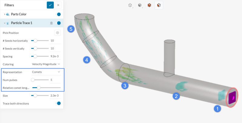
Figure 20: With this configuration, 5 groups (or Pulses) of comets are visible in the domain. The length of each comet is controlled by its velocity and the Relative comet length.
Plot Over Path
The Plot-over-path filter helps visualize how simulation quantities vary over a desired path within the simulation domain. This path is created using sample points added by the user.
Settings:
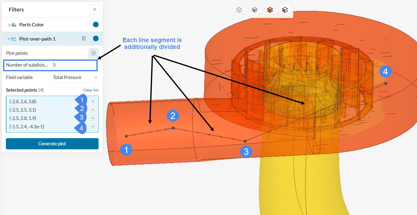
- Pick points: Allows manual picking of points on the exposed domain surface.
- Number of subdivisions: Enter the number of subdivisions that parts the line into segments and creates additional intermediate equidistant subpoints.
- Field variable: Select the simulation quantity to plot over the desired path.
- Selected points: Displays the coordinates of points picked manually.
- Generate plot: Once the settings are configured, click this button to create the plot.
Once the settings are acceptable, hit the ‘Generate plot’ button to generate the plot. The plot is displayed as follows:
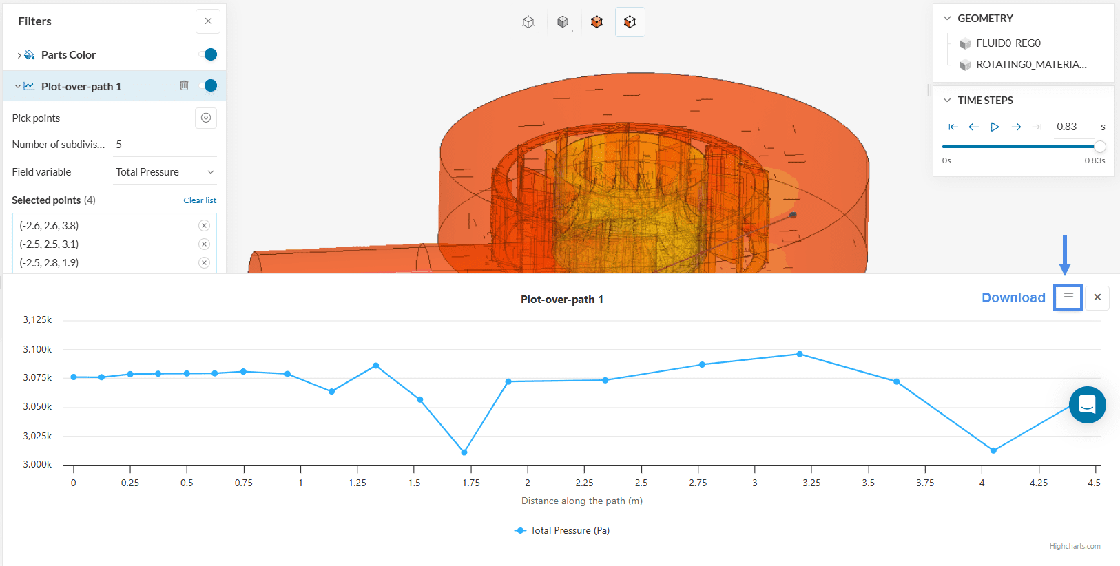
The generated plot can also be downloaded in different file formats for further processing.
Key highlights:
- Multiple line segments can be chained by continuously adding control points.
- The filter works on volumes, faces, and cutting planes.
- Multiple instances of the filter can be used in the same project.
- For transient simulations, plots update automatically across time steps.
- Hovering over control points in the list highlights them on the model.
- The plot refreshes on-the-fly when points are added or modified.
Plotting over surface
The sample points are always connected by straight lines. They do not conform to the CAD model’s surface geometry. Intermediate sample points created by subdivisions may pass through the CAD body or lie outside the geometry. In such cases, the resulting gaps will appear in the generated plot.
Rotational
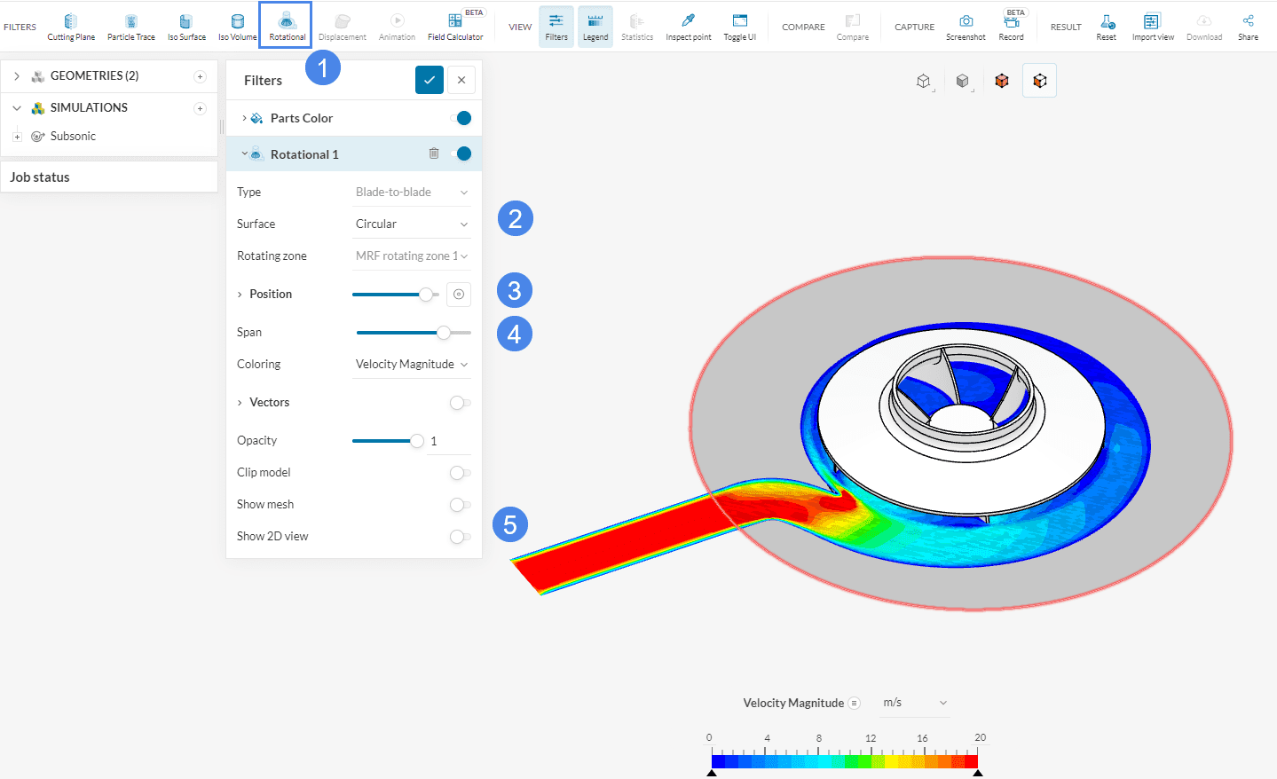
A Rotational view allows the user to inspect a rotational region by creating a cascade blade-to-blade view, this helps to better understand the flow in between blades. The filter also allows for an unwrapped rectangular 2D view of the circular cutting surface through the rotating region.
To create a rotational view add a new Rotational filter. The representation of the field values can be done on a circular surface. For a circular surface, define the position of the surface as well as the radial span to create a section at specific points of the rotating geometry. The user can also display vectors, clip through the model, or display the generated mesh on the circular surface.
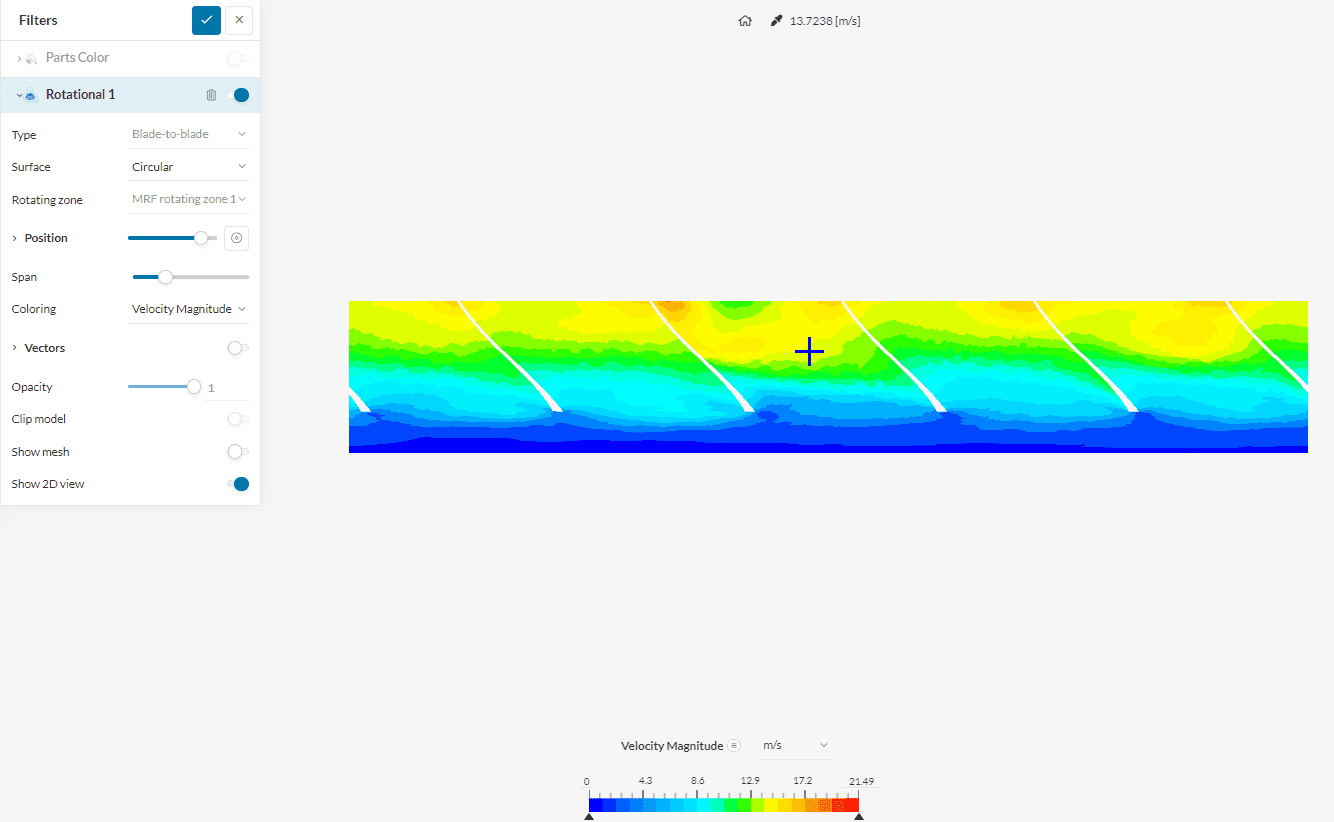
Show 2D View
In addition, it is possible to unwrap the circular surface into a two-dimensional rectangular surface to achieve a view of each blade side by side. This view is called the Cascade view. Cascade view is used by turbomachinery designers and engineers to analyze near-blade flow profiles such as recirculation, flow separation, pressure, and suction and understand flow passage through each stage of compressors, pumps, or turbines.
An example of this unwrapped view can be seen below. Within this view, the value of the field function based on the cursor position will be displayed at the top.
Displacement
With the displacement filter, the deformations appearing in the CAD as a result of boundary conditions in a structural simulation can be visualized. Following is an animation that shows the use of Scaling factor to magnify the displacements in a bracket for easier visualization:

Animation
The animation filter is often used on two occasions:
- In combination with a particle trace filter
- To animate the results of a transient analysis
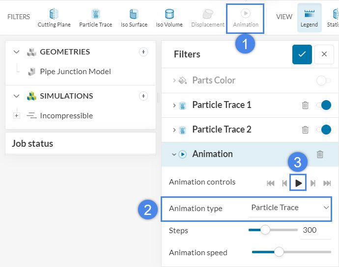
After setting the Animation type to Particle Trace, we can simply click on the ‘Play’ button, to generate an animation of the streamlines. Note that you can change the number of Steps, to control the number of frames of the animation.
Recording an Animation
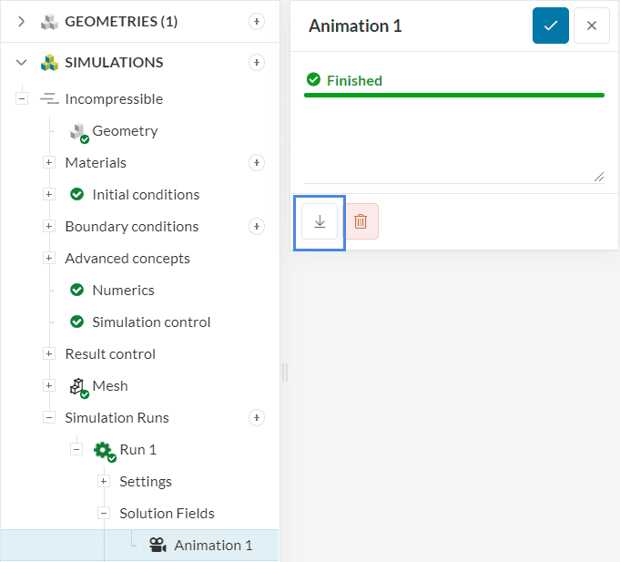
After creating an animation, you can generate a GIF of the result directly in SimScale. To do this, create a ‘Record’ filter and press ‘Record animation’ when you are satisfied with the settings.
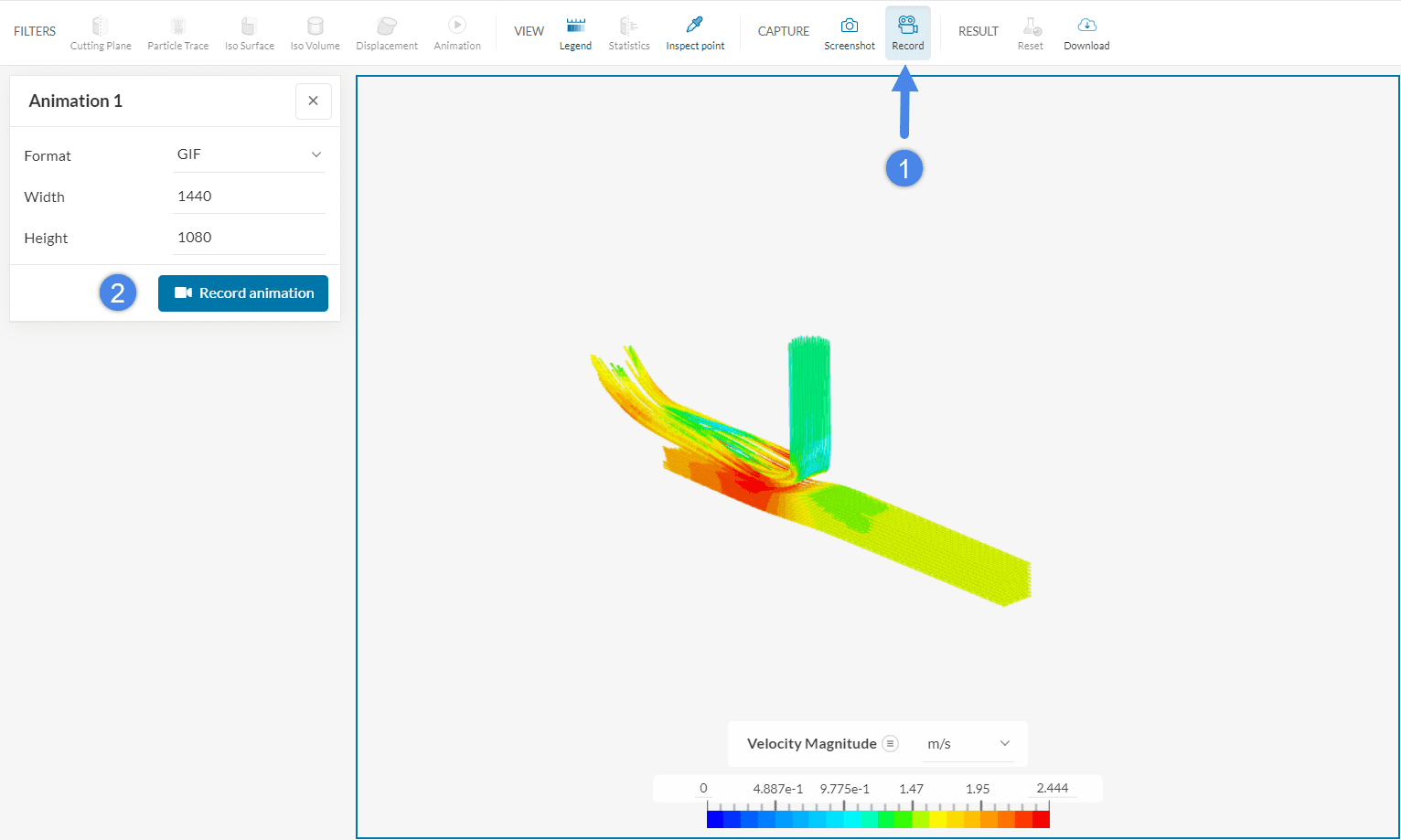
After the animation finishes rendering, it is available for visualization/download under the simulation run.
Please note that the Record filter is currently in beta test.
Important
The Record option will be unavailable (grayed out) in the following cases:
- You have read-only access, meaning that you do not own the project you are processing.
- The solver you are using for this simulation is Multi-purpose.
- The result is in Compare mode.
- The simulation is not finished yet.
- No more than one step is saved in the Post-Processor, and, it doesn’t include Particle Trace.
- A new field has been created through the Calculator.
- You have activated the selection of the position for the Particle Trace seeds, but you have not completed that step yet.
- The Post-processor is still loading.
Field Calculator (Beta)
The Field Calculator filter, currently in a beta testing phase, allows the user to use fields, functions, and operators to obtain completely new fields to post-process.
For example, you can use the field calculator filter to obtain the total gauge pressure inside the pipe -please proceed as follows:
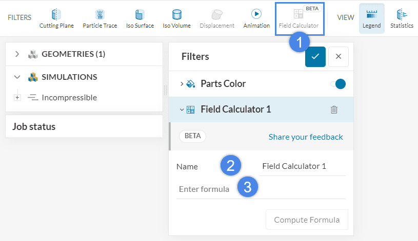
- Click on ‘Field Calculator’ to create a new filter
- The Name is an arbitrary name of the new field that you are calculating (e.g. ‘Total gauge pressure’)
- Under Enter formula, you can define the formula used to obtain the new field
For the total gauge pressure, the following formula will be used:
$$P_0 = P + 0.5 \rho V^2 \tag{1}$$
Where \(P_0\) is the total pressure, \(P\) is the static pressure, \(\rho\) is the density of the fluid, and \(V\) is the local velocity magnitude.
To add a term to a formula (be it a scalar, a vector, or an operator), you can start typing in the Enter formula field. A drop-down window will appear with options to choose from – simply click on the option to confirm. Looking at formula 1, the first term to define is the static pressure, therefore we can do as follows:
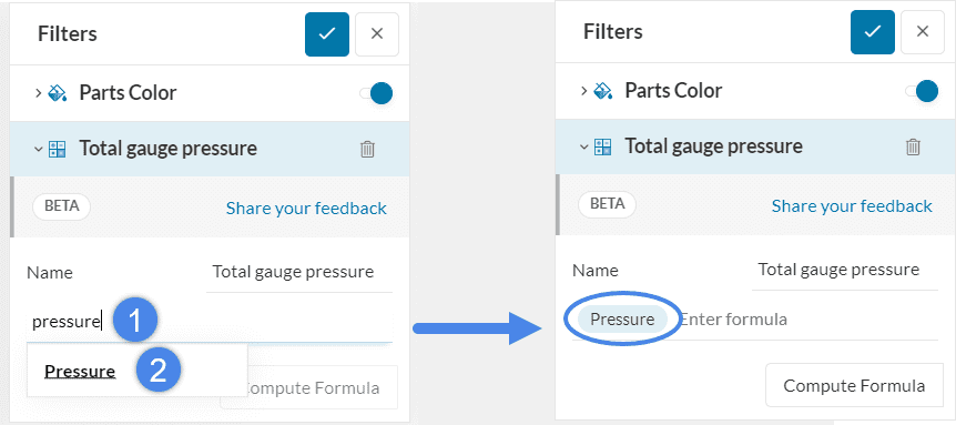
- The first term in the total pressure formula is static pressure. Therefore, you can type ‘Pressure’ in the Enter formula field
- A menu will appear with options. Pick ‘Pressure’ from the menu to add it to the formula. Now you can repeat the same process to add the other terms.
Once the formula configuration is finished, it will look like the image below:
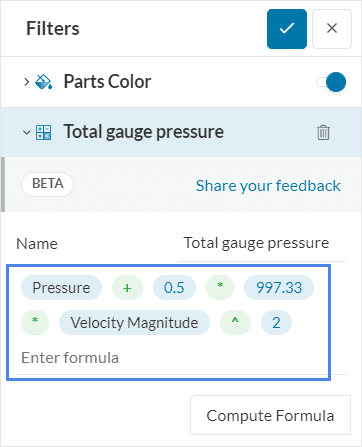
Once the formula is finished, you can click on ‘Compute Formula’ to proceed. A new field is created and will be available for visualization in the post-processor.
Save and Manage View
Simulating a project and drafting a professional report might require recreating the same angles and screenshots for all the visual results. To take advantage of this consistency in your animations and images use the Save view filter where you can save and manage views across different simulation runs within the same project as well as across different projects.
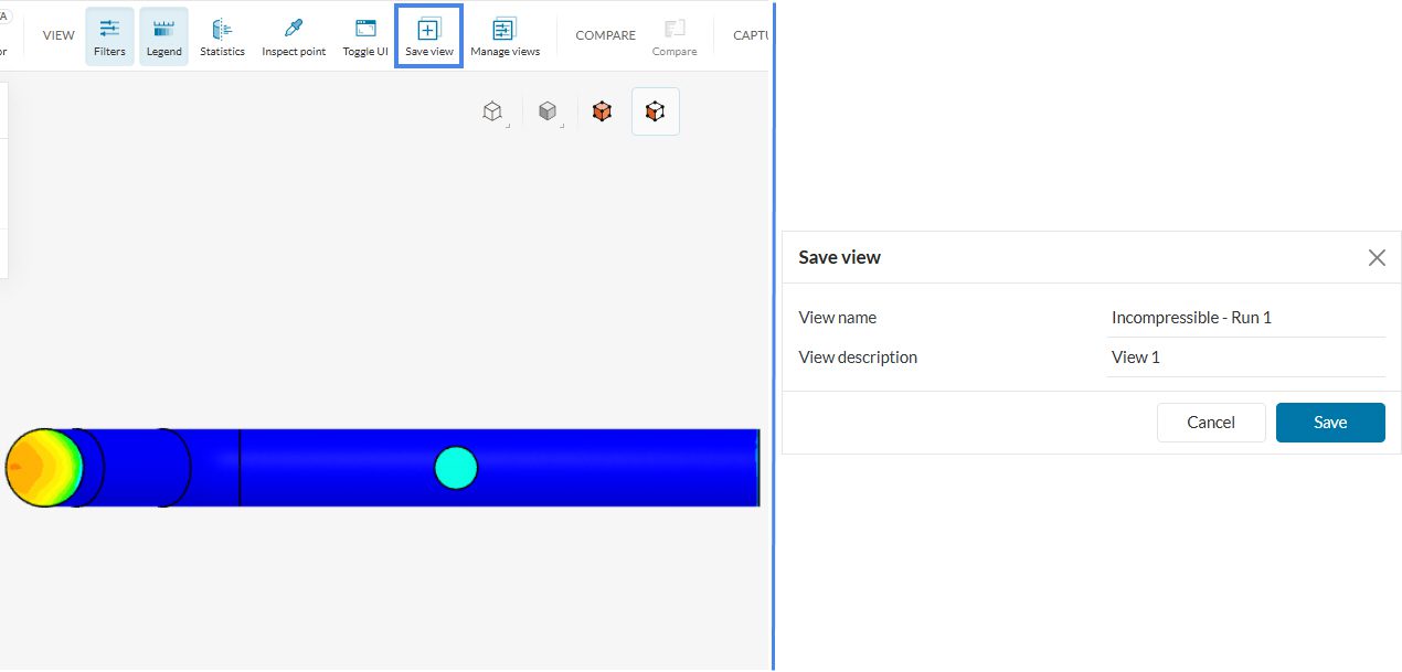
Once a view is finalized click on ‘Save view’ and provide a name and description for the view before saving it.
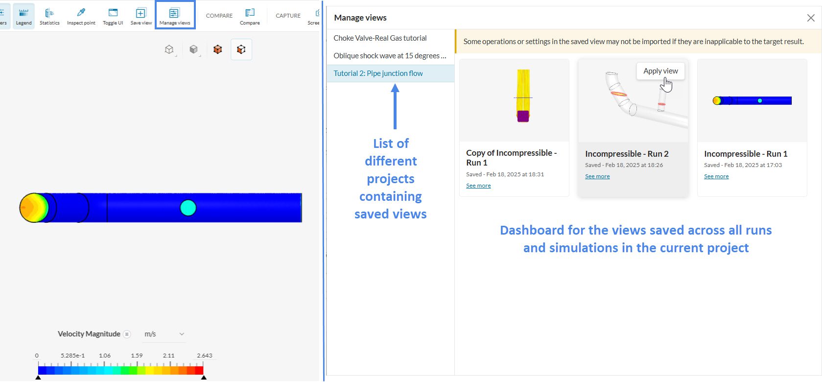
Using Manage view one can sort through the pre-saved views across the same or different runs from the current project or different projects. Select a view tile for more details or simply click ‘Apply view’ to apply that view including the filters.
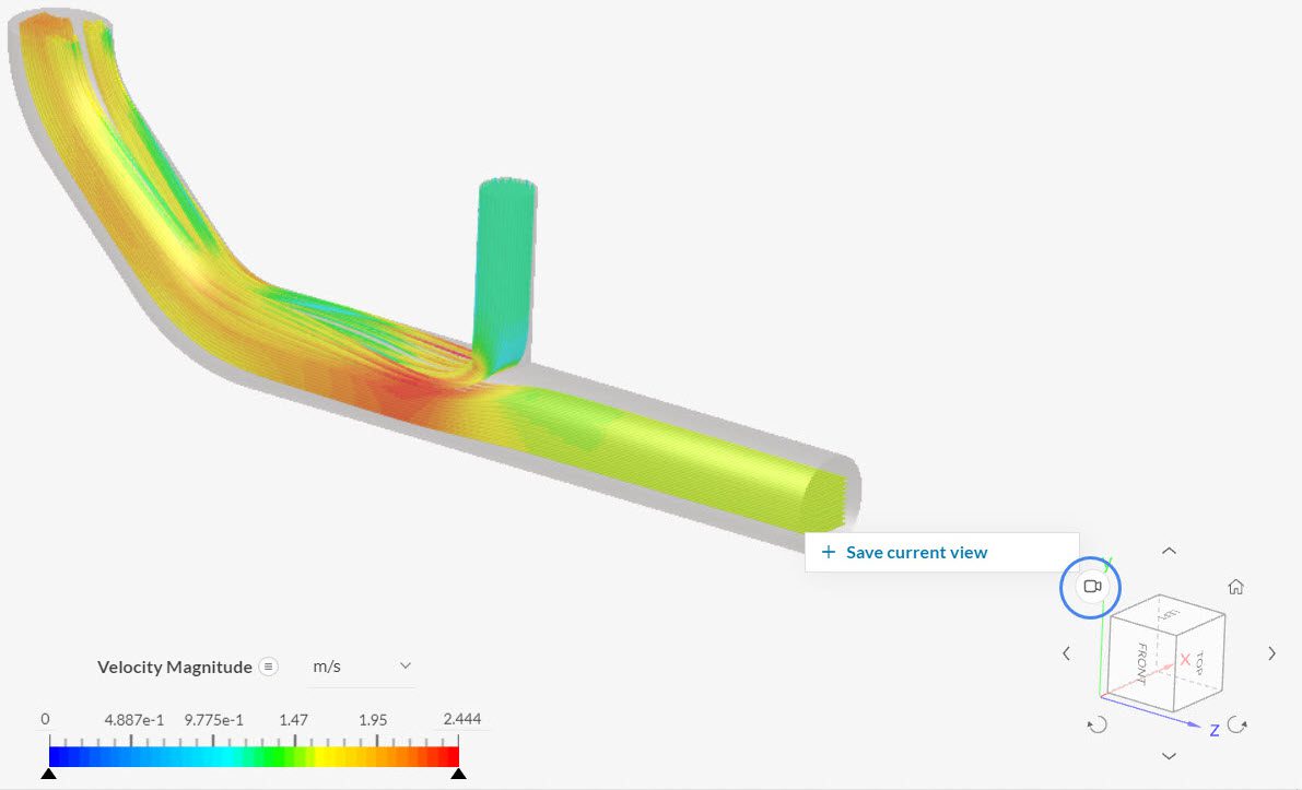
Custom Camera Position
The Custom camera position feature is similar to save view except that it only mimics the view angle and not the filters applied. This also makes it quicker. Note that views from other projects cannot be applied. This feature can be seen at the top left of the orientation cube.
To learn more about this handy feature refer to our knowledge base article.
Compare
The Compare tool allows to visualize the result fields from two different simulation runs side by side, with synchronized viewers and filters. To activate the side-by-side view:
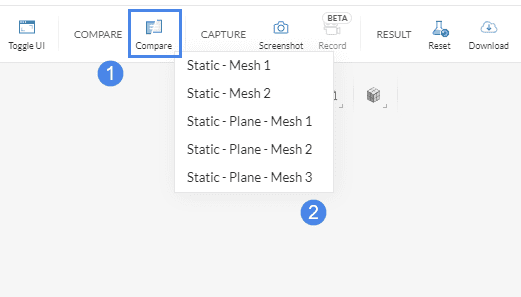
- Select the ‘Compare’ command from the filters bar.
- Select the simulation run you want to compare to from the drop-down list.
The operation applies the same filters to both results and by default synchronizes the camera views. If you rotate, zoom, or pan one of the views, the other view is updated correspondingly. The figure below shows an example comparison view:
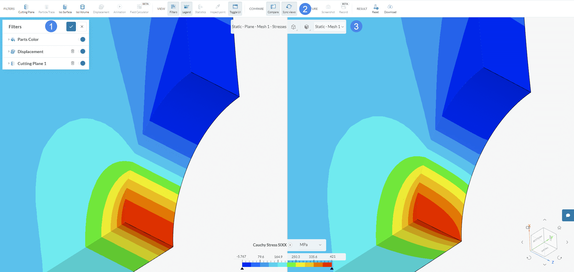
There are also options to:
- Manage the applied filters, simultaneously for both result fields.
- The Sync views button allows to toggle the camera synchronization on and off.
- Change the selected results to compare from the list.
Warning
Both of the views that are displayed will correspond to the latest timestep of their simulations, and this can not be adjusted. Also, it is not possible to select and hide faces/parts that belong to the second view (on the right). Finally, the syncing of the views is always controlled by the left one, and implemented to the right.
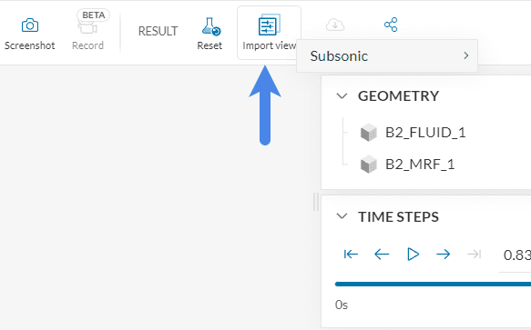
Import View
Much like the Compare feature, Import view is only available in projects with more than one simulation. With import view, you can copy the post-processing state from another simulation to the current post-processor instance:
The following settings are copied:
- Filters, where applicable
- Fields, where present
- View (camera) settings
- Global color
- Part visibility, for matching topologies
Download the Results
The workflow on the SimScale platform is kept as modular and as open as possible, allowing you to use a third-party post-processing platform, such as ParaView, to analyze the results. It has been discussed in detail here:
Troubleshooting
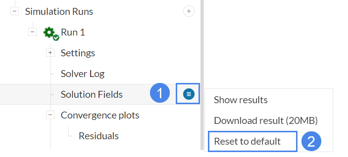
In case of problems with the post-processor, please reset it to the default settings. There are two ways to do this :
- Within the simulation tree, navigate to Solution fields and click on the hamburger button and then select ‘Reset to default’:
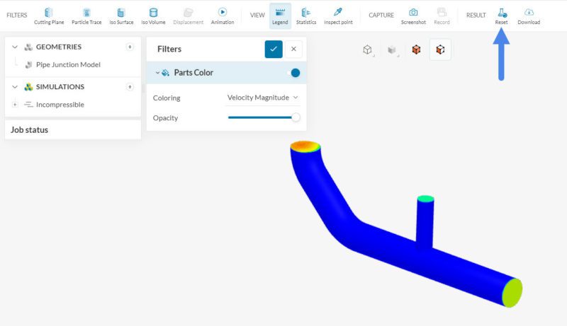
- Alternatively, in the online post-processor window, simply click on the ‘Reset’ button:
Feeling Inspired?
If you would like to use these post-processing filters and tools in different projects, make sure to check our step-by-step tutorials. Each tutorial contains a post-processing section with new ideas and combinations of filters.
Furthermore, it is also possible to readily post-process thousands of projects from other users in the Public Projects section.
Last updated: August 29th, 2025
Did this article solve your issue?
How can we do better?
We appreciate and value your feedback.


