Frequency Analysis

The Frequency Analysis simulation type allows the computation of natural (under no external load excitation) frequencies of oscillation of a structure and the corresponding oscillation mode shapes. The resulting frequencies and deformation modes are dependent on the geometry and material distribution of the structure, with or without the displacement constraints. In SimScale, the Code Aster solver is used to perform the frequency analysis.

The results from a frequency analysis enable you to evaluate the overall rigidity of your structure, as well as the rigidity of local regions. The lower frequencies of oscillation can be used as input for the seismic or wind load assessment and computation of structures. Also, in parts and structures subjected to variable frequency loads, the fundamental frequencies are used to avoid resonance between the natural oscillation modes and the applied load.

example vibration mode frequency analysis — Figure 1: Natural vibration mode shape of a quarter ring

Creating a Frequency Analysis

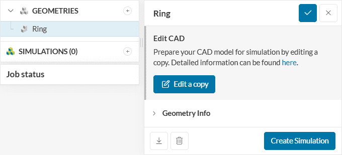
To create a frequency analysis, first select the desired geometry from the top of the simulation tree on the left, and then click on ‘Create Simulation‘:

creating a new frequency analysis simulation — Figure 2: Create simulation for the selected geometry

The simulation library window will appear with all the available analysis types:

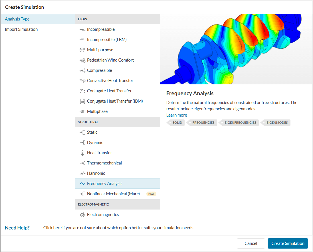
simulation library frequency analysis — Figure 3: SimScale simulation library. Select *Frequency Analysis* and click on ‘**Create Simulation**‘.

Select ‘Frequency Analysis’ from the list and confirm the choice by clicking on the ‘Create Simulation‘ button. A new element will appear in the simulation tree with all the available settings:

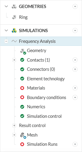
simulation tree frequency analysis — Figure 4: Frequency analysis simulation tree.

In the next sections, the different simulations settings that need to be defined to run the simulation are described:

Global Settings

The global settings are accessed by clicking on the simulation name, in this case, ‘Frequency Analysis’, from the simulation tree. For this type of analysis, there are no further parameters to change. For more information, please refer to the global settings page.

Geometry

The geometry panel contains the CAD model used for the simulation. Details of CAD handling and manipulation are described in the pre-processing page. Additionally, if you are facing problems with CAD complexities and uploading then it is advised to visit this documentation.

Contacts

Geometrical models consisting of multiple bodies require connections to be defined on faces that make contact. The possible choices are:

Bonded contact: The master faces are rigidly connected to the slave faces, creating continuity on the deformation and compliance of forces.
Sliding contact: The master faces are connected to the slave faces, but the local tangential displacements and forces are not transmitted.

Upon creating the simulation, all interfaces are automatically detected and defined as bonded contacts, but they can be further configured. Read more information about contacts here.

Important

The default bonded contact method can introduce some inaccuracies in 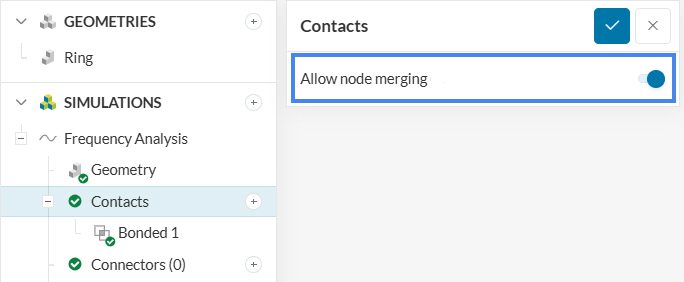Frequency analysis results. More precisely, it can prevent some rigid body modes to be detected in a free-free modal analysis. We recommend using ‘Allow node merging’ option, also called conformal meshing, to obtain the most reliable results, specially in such case.

Conformal Contact Mesh Node Merging Option — Figure 5: Allow node merging to generate conformal meshing in a free-free modal analysis.

Element Technology

Element technology refers to the numerical formulation for the solid finite element used in the simulation. This includes the mesh order, reduced integration, and mass lumping.

Materials

Select a material from the materials library or customize the material model with your own parameters. Then, assign the created material models to each volume in the geometry. Please see the materials section for more details.

Boundary Conditions

In frequency analysis, you will find that only displacement constraints are available. This is due to the assumption that the body is vibrating without the effect of any external load. If the analysis aims to compute the free body motion modes of vibration, no displacement restriction must be imposed. For an overview of all the boundary conditions available, please check this page.

Numerics

The parameters of the modal and linear equations solvers are controlled in Numerics. For most cases, the default choices should be enough to get accurate results. You can find more information on numeric settings in the following blog post:

How to Choose a Solver for FEM Problems: Direct or Iterative?

Simulation Control

The computation mode is specified under Simulation control. The available choices are:

First modes: Compute the first ‘Number of modes’, according to the lower vibration frequencies.
Frequency range: Compute all the modes in the band of frequencies ranging from Start frequency to End frequency.

If there is a need to compute the free body motion modes, the ‘Start frequency’ should be a small negative number, such as -0.1. Additionally, if the objective of the study is to determine the free body motion modes, it is recommended to enable node merging within the Contacts tab for improved accuracy, as shown above in Figure 5.

Result Control

Under result control, the user can select desired output fields from the computation. In the case of frequency analysis, the only available field is displacement. It is important to note that the magnitude of the displacements only has a relative meaning and no physical interpretation.

Mesh

For a frequency analysis, the Standard and Tet-dominant meshing algorithms are available. For more information about meshing in SimScale, please refer to the dedicated page.

Results

After a successful simulation run, you will find the results in the following items:

Solution Fields

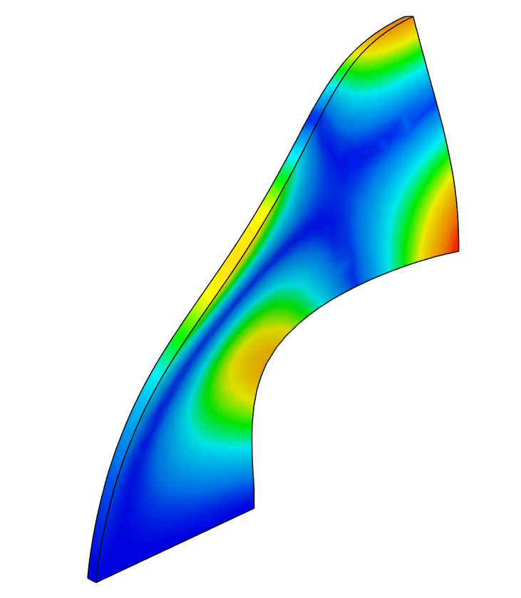
Opens the online post-processor to visualize the deformed shape for each computed natural frequency of oscillation. Notice that the numerical values of the deformations not absolute, thus they do not contain any physical meaning, besides the relative deformations in the mode shapes.

The magnitudes of the deformations are normalized according to a ‘Translational-Rotational’ criteria. This means that all the computed deformations are divided by the largest value among all of the degrees of freedom, to achieve a maximum value of 1 on the component with highest deformation, and the other components are scaled proportionally.

Tables

Presents a table (labeled ‘Statistical data’) with the numerical results from the frequency analysis. The results are presented as a list of:

Eigenmode number,
Eigenfrequency, the oscillation frequency for the mode,
Modal Effective Mass (MEM), in DX, DY and DZ directions,
Normalized Modal Effective Mass, in DX, DY, and DZ directions,
Cumulative Normalized Modal Effective Mass, in DX, DY and DZ directions.

For a total of 11 data columns. The result data can be downloaded in a text CSV table form.

Plots

Presents the results of the frequency analysis as line plots for the following quantities:

Eigenfrequency plot, shows the natural frequency vs mode number.
Modal effective mass plot, shows a plot for each direction vs mode number.
Accumulated normalized modal effective mass plot, shows a plot for each direction vs mode number.

What are these modal quantities?

For an explanation of what modal effective mass quantities are, its derivatives and applications, please refer to this page.