Initial Conditions
With initial conditions, users can define the initialization of various parameters in their system. The fields to initialize depend on the analysis type, physics, and also time dependency.
To set the initial conditions of your simulation, simply navigate to the Initial conditions tab in the simulation tree. By expanding the tab, you will find a list of the fields to initialize.

Before going through the lists of fields, let’s see how the initialization of the fields impacts steady-state and transient simulations.
Time-Dependency
Initial conditions define the starting values for each solution field. Therefore, they play a vital role in the stability and computing time of steady-state simulations. To ensure a good convergence rate for a steady-state simulation, it’s a good practice to initialize the domain close to the expected solution.
In the case of transient analysis, the initial conditions are vital for the setup. They define the state of the system when time is equal to zero and will play a major role in the simulation. For instance, if we are studying the transient cooling effects of a piece of metal, there is a huge difference between initializing the metal part at 350 \(K\) or 800 \(K\).
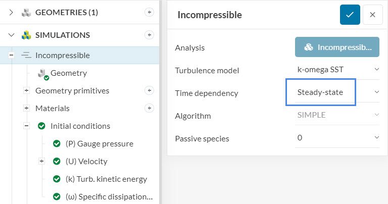
The time dependency definition of a simulation is set under the Global settings:
Methods of Initialization
In SimScale, there are two main methods to initialize the domain: global and subdomain initialization.
Global Initialization
As the name suggests, the global initialization applies the initial condition to the entire domain.
Global initialization is the most commonly used type of initialization. However, for some simulations, we may choose to initialize a portion of the domain with a different value. In such cases, the subdomain initialization is very useful – find more details below.
Subdomain Initialization
The subdomain-based initialization allows users to initialize a field in a specific region of the domain called a subdomain. Note that the subdomain initialization overrides the global initialization:
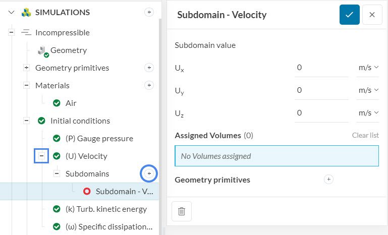
A subdomain can be defined using a geometry primitive or by assigning a volume region. For a detailed guide on subdomain initialization, please refer to this tutorial.
Below, we will go through all parameters that can be initialized in SimScale. Please note that the list varies based on the analysis type and physics of your simulation.
Initial Conditions Types
Depending on the analysis type and physics, SimScale will require the initialization of different fields. Find below the fields available.
Fluid Dynamics
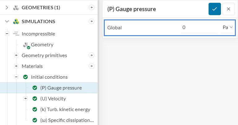
Pressure
Note that the input pressure may be different, depending on the analysis type. For example, an incompressible analysis requires gauge pressure, whereas a conjugate heat transfer simulation with compressibility enabled requires the absolute modified pressure. The pressure field may be initialized with global and subdomain definitions.
Velocity
For velocity, you can define both global and subdomain initialization.
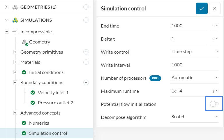
Note that there is a third type of velocity initialization available for some analysis types, named potential flow initialization. This setting initializes the velocity field with a potential flow, which can enhance the stability of velocity-driven flows.
Turbulence Parameters
Turbulent kinetic energy (\(k\)), Specific dissipation rate (\(\omega\)), and Dissipation rate (\(\epsilon\)) are related to the level of turbulence in the domain. As the name suggests, these parameters are only available for initialization if you are using the k-epsilon, k-omega, or k-omega SST turbulence models in the global settings.
In terms of initialization, \(k\) and \(\omega\) are required for the k-omega and k-omega SST turbulence models, whereas \(k\) and \(\epsilon\) are required for the k-epsilon model. For a good rule of thumb of the global initialization of the turbulence parameters, please refer to this post.
Modified Turbulent Viscosity
The parameter \(\widetilde{\nu}\), also known as modified turbulent viscosity, is exclusive to the LES Spalart Allmaras turbulence model. Find on this page a rule of thumb for its initialization.
Passive Scalar 1
The passive scalar initialization is related to the passive scalar transport model, which is available for incompressible and convective heat transfer analyses. Both subdomain and global initializations are available.
Temperature
Some analysis types, such as convective heat transfer and conjugate heat transfer require temperature initialization, which can be done both globally, and via subdomains. For steady-state simulations, the best practice is to initialize the domain close to the expected solution.
Turbulent Thermal Diffusivity
The turbulent thermal diffusivity \(\alpha_t\) is a parameter that is automatically calculated based on the turbulence parameters, density, and thermal properties of the material.
It is available for global initialization in analysis types that involve temperature.
Eddy Viscosity
In CFD, the Eddy viscosity has two main variants: turbulent dynamic viscosity (also known as \(\mu_t\)) and turbulent kinematic viscosity (also known as \(\nu_t\)).
In SimScale, the eddy viscosity always refers to the turbulent dynamic viscosity, and can be calculated by Equation 1:
$$Eddy\ viscosity = \frac{\rho k}{\omega} \tag{1}$$
Where \(\rho\) is the density of the fluid. \(k\) and \(\omega\) are the turbulent kinetic energy and specific dissipation rate, respectively.
Phase Fraction
The phase fraction initialization is exclusive to the multiphase analysis type. With this setting, the user can define global or subdomain initialization for both phases being simulated.
Solid Mechanics
Generally speaking, only nonlinear or transient solid mechanics analyses require initialization. Furthermore, it is worth noting that all initial conditions for solid mechanics accept subdomain initialization. Find below a list of the parameters available.
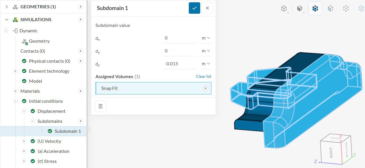
Displacement
Displacement initialization is available for nonlinear static, nonlinear thermomechanical, and dynamic analyses. It is worth mentioning that a table input method is also available for global initialization.
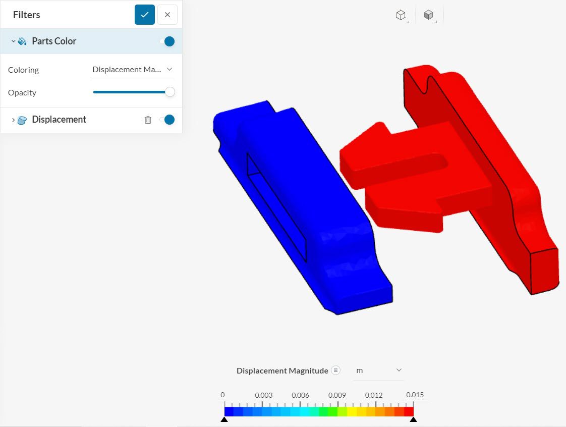
The displacement initialization is useful for translating the initial position of certain parts for the simulation. In the example below, the initial CAD model for a snap-fit analysis has both parts connected. By applying a displacement initial condition to one of the parts, we can disconnect both parts without changing the CAD model:
As a result, the parts are separated in the initial state of the simulation:
Stress
The definition of stress initialization requires all normal and shear components of stress, as in Figure 8:
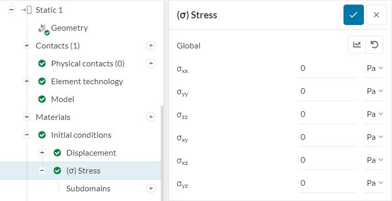
The normal components of stress are indicated with two of the same letters in the subscript (xx, yy, and zz) whereas the other entries represent shear stresses (xy, xz, and yz).
Velocity
For many dynamic simulations, such as drop tests, the initialization of velocity is very important.
As a reminder, dynamic analyses are inherently transient and consider inertia effects. Therefore, the initialization of the domain plays a major role in the solution.
For an example of a simulation that initializes velocity, please check out this tutorial.
Acceleration
Like velocity, this field is only available for dynamic and thermomechanical simulations (in Dynamic mode for the Inertia effects).
Temperature
The only two types of FEA analysis types that model temperature are thermomechanical and heat transfer. Please note that the initialization of temperature is only required for transient analysis.
Last updated: February 20th, 2026
Did this article solve your issue?
How can we do better?
We appreciate and value your feedback.
What's Next
Boundary Conditionspart of: Simulation Setup


