Result Control – Structural Analysis
The result control fields for structural simulations depend on the chosen analysis type. A list of all the available structural analysis types can be found on the analysis types page. Although the availability of each result control item can vary, the generally available options are as follows:
The different result control items can be applied over a sample point, specific geometry entity or the whole geometry, as described below:
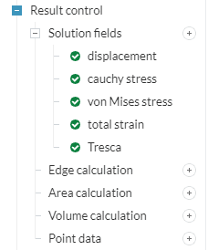
- Solution fields: Fields to be retrieved for the complete geometry. Details on the available fields and analysis types are given below.
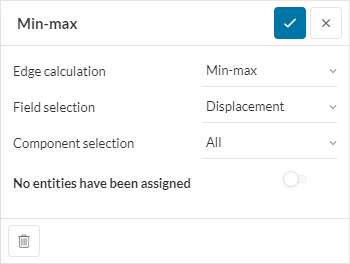
- Edge calculation: Computation of statistics of a given field over all the nodes belonging to the assigned edge(s)
- Area calculation: Computation of statistics of a given field over all the nodes belonging to the assigned face(s)
- Volume calculation: Computation of statistics of a given field over all the nodes belonging to the assigned volume(s)
- Point data: Sampling of a given field in a location. The location is specified by creating a geometry primitive point, through its (X, Y, Z) coordinates or by picking a position from the viewer. The value of the field at the given location is computed by interpolation of the closest mesh nodes.
For the Solution fields, the output data can be visualized and examined using the online post-processor or downloaded to use a local post-processor such as ParaView. On the other hand, for the computation of statistical data, the results are given in graph format, with the option of downloading the data in table format.
The available statistic computations for the geometrical entities assignments are summarized below:
- Min/Max: Minimum and maximum values for the specified field are computed over all the mesh nodes belonging to the assigned geometry, e.g., all nodes belonging to a particular face. If the field contains multiple components, such as vector or tensor quantities, select the ‘All’ components option to obtain the minimum and maximum values for each individual component.
- Average: Average value of the specified field is computed over all the mesh nodes belonging to the assigned geometry (edge, face or volume). If the field contains multiple components, such as vector or tensor quantities with the ‘All’ components option selected, the sum is reported for each individual component.
- Sum: Summation of the values of the specified field over all the mesh nodes belonging to the assigned geometry (edge, face, or volume). If the field contains multiple components, such as vector or tensor quantities, you can select the ‘All’ components option to obtain the sum of each individual component.
The available solution fields according to the different analysis types and their definitions are documented below:
Static Analysis
For a Static linear or nonlinear simulation, the following solution fields and categorizations are available:
- Displacement:
- Nodal displacements: Displacement vector for each node in the model, expressed in global components DX, DY, DZ.
- Force:
- Reaction Force: Reaction forces computed on the nodes of the model. The field is non-zero only on faces with imposed displacement boundary conditions, such as Fixed support, Fixed value, or Symmetry plane. Expressed in global components X, Y, Z.
- Nodal Force: Applied forces as computed on the nodes of the model. The field is non-zero only on entities with load boundary conditions, such as Force, Pressure, etc. Expressed in global components X, Y, Z.
For a detailed understanding of the difference between nodal and reaction forces see here: Nodal vs Reaction Force
- Moment:
- Reaction Moment: Computed from the reaction forces \(\vec{F}\) at the nodes, and the lever arm vector \(\vec{r}\) pointing from a reference point to the node, e.g. \(\vec{M} = \vec{r} \times \vec{F} \). Just like the reaction force, this field is non-zero only on faces with imposed displacements. As a vector, it is expressed in global components X, Y, and Z, and interpreted according to the right-hand rule.
- Nodal Moment: Computed from the nodal forces and the lever arm vector pointing from a reference point to each node. Like the nodal forces, this field is only non-zero on entities assigned to load boundary conditions. As a vector, it is expressed in global components X, Y, and Z, and interpreted according to the right-hand rule.
- Strain:
- Total strain: Strain tensor computed from the nodal displacement, under the theory of small deformations. Expressed in the global components for axial (EPXX, EPYY, EPZZ) and shearing (EPXY, EPXZ, EPYZ).
- Principal strain: The set of three values and corresponding directions at which axial strains are maximized. The three principal axial strains are given, ordered from lower to higher value (PRIN_1, PRIN_2, PRIN_3). For each principal strain, the corresponding direction is given as vector components (VECT_1_X, VECT_1_Y and VECT_1_Z for PRIN_1, and so on for directions 2 and 3).
- Total nonlinear strain: Strain tensor of Green-Lagrange, under the theory of large deformations. Expressed in the global components for axial (EPXX, EPYY, EPZZ) and shearing (EPXY, EPXZ, EPYZ).
- Total equivalent plastic strain: Equivalent strain of von Mises, corresponding to the plastic region of the stress-strain curve. A Zero value of this field means that plasticity has not occurred in the material (or that the material model does not consider plasticity).
- Unelastic strain: Named ‘plastic strain’ in the SimScale post-processor. Corresponds to the plastic component of the total nonlinear strain tensor, computed by subtracting the linear elastic strain. Expressed in the global components for axial (EPXX, EPYY, EPZZ) and shearing (EPXY, EPXZ, EPYZ).
- Stress:
- Cauchy stress: Stress tensor computed from the deformations and the material properties. Expressed in the global components for axial (SIXX, SIYY, SIZZ) and shearing (SIXY, SIXZ, SIYZ).
- Principal stress: The set of three values and corresponding directions at which axial stresses are maximized. The three principal stresses are given, ordered from lower to higher value (PRIN_1, PRIN_2, PRIN_3). For each principal value, the corresponding direction is given by vector components (VECT_1_X, VECT_1_Y and VECT_1_Z for PRIN_1, and so on for directions 2 and 3).
- Tresca stress: Equivalent shear stress, computed from the principal stresses. It is related to the maximum shear stress theory of yielding.
- Von Mises stress: Equivalent axial stress, computed from the principal stresses. It is related to the critical distortion energy theory of yielding.
- Signed von Mises stress: The von Mises stress, multiplied by the sign of the trace of the Cauchy stress tensor. It is useful to find out which points in the material are under tension (positive sign) or compression (negative sign).
- Contact:
- Pressure: The pressure distribution applied on a surface due to the action of an active physical contact. The pressure is computed at each node in the surface starting from the Cauchy stress tensor \(\sigma\) and the normal vector computed from the deformed geometry \(\vec{n}\): $$ p = (\sigma \cdot \vec{n}) \cdot \vec{n} $$
- State: Retrieves a set of fields related to the state of the physical contacts. In the post-processor, it is identified as ‘Contact Results’, with the following components:
- Contact State: Takes the value of 0 for no contact, 1 for adherent contact (only possible if friction is taken into account), 2 for sliding contact, and 3 for interpenetration.
- Contact Gap: The distance between a node in the slave surface and the closest element in the master surface, projected to the normal.
- Contact Normal Force: Magnitude of the normal reaction force due to the contact.
Dynamic Analysis
For Dynamic simulations, all the solutions fields from static analysis are available, in addition to the following:
- Velocity:
- Nodal velocities: Velocity vector for each node in the model, expressed in global components X, Y, Z.
- Acceleration:
- Nodal accelerations: Acceleration vector for each node in the model, expressed in global components X, Y, Z.
Heat Transfer and Thermomechanical Analysis
In a Thermomechanical analysis, the available fields are the same as in a Static or Dynamic analysis, depending on the choice of Inertia effect on the global analysis parameters. In addition to those, the following thermal fields are available:
- Temperature: Temperature scalar value for each node in the model.
- Heat Flux: Heat flux vector for each node in the model, expressed in global components X, Y, Z. It has units of energy per unit of time per unit of area \(J / (s \cdot m^2)\)or units of power per unit of area \(W / m^2\).
- Heat Flow: Available as an Area calculation, retrieves the total heat per unit time (\(J/s\)), or power (\(W\)), leaving or entering the domain through the selected faces. This field is computed as the integral of the Heat Flux over the selected surface.
Frequency Analysis
For Frequency analysis, the only available solution field is the nodal displacements (see the description above under Static for details). In this case, the computed displacement magnitudes do not have a physical meaning but are relative to each other, and normalized to achieve a maximum value of 1 \(m\) on the component (X, Y or Z) with the largest deformation.
Modal Effective Mass (MEM)
For the tables and plot results, the Modal Effective Mass (MEM) is introduced, alongside some derived quantities, that are of interest for vibration analysis of the model. Here is the definition of each of these quantities:
- Modal Effective Mass (MEM): The modal effective mass represents how much mass is moving in each of the coordinate directions – DX, DY and DZ for a given mode of natural oscillation. This quantity is useful to measure the importance of a mode in a base excitation scenario, because it indicates the amount of mass that will be excited (and probably enter in resonance) with the base moving in a determined direction.
- Normalized Modal Effective Mass: The MEM is normalized to the total mass of the model, in order to judge the importance of each mode: a value of 0 means no importance while a value of 1 means that the whole mass would oscillate under a base excitation in this direction. This quantity also helps to separate global from local vibration modes by ordering from higher to lower values.
- Cumulative Normalized Modal Effective Mass: A common question in vibration analysis is: how many modes are important for my model? This question is answered by adding (accumulating) the normalized modal effective mass of the modes, ordered in increasing frequency: as our sum adds up closer to 1, we can tell that the considered modes cover most of the oscillating mass in our model. This is specially useful when performing a dynamic analysis (transient or harmonic) on modal base, where we need to select the number of natural modes to use for the modal base, for example by selecting the first n modes that cover at least 80% of the oscillating mass in every direction.
Harmonic Analysis
In a Harmonic analysis, the following result fields are available. The definition of each field is the similar as those given for the Static and Dynamic types.:
- Displacement
- Absolute
- Relative
- Force
- Reaction Force
- Nodal Force
- Strain
- Total strain
- Stress
- Cauchy stress
- Von Mises stress
- Von Mises stress (Max over Phase)
- Velocity
- Acceleration
- ERP Density (Equivalent Radiated Power)
For a harmonic analysis, since the fields are a function of the excitation frequency and not time, each field is modeled with a phasor. The resulting field can be retrieved in one of two representations:
- Magnitude and phase: The physical magnitude of the field and the delay with respect to the applied load, in terms of the phase angle in units of radians.
- Real and imaginary: The components of the complex number representing the phasor. The components have no physical meaning on their own, thus we recommend using the magnitude and phase representation by default.
Important
The default Von Mises stress result control outputs a computation based on the peak stress components at a given frequency, which results in a conservative estimation of the peak value of the Von Mises stress. On the other hand, the Von Mises stress (Max over Phase) result control reports the maximum Von Mises stress experienced taking the phase angles into account for a given frequency.
As such, max over phase results are preferred in case of simulation setups involving material damping or stress components at phase angles different than 0.
References
Last updated: October 29th, 2024
Did this article solve your issue?
How can we do better?
We appreciate and value your feedback.


