Simulation Control for Structural Analysis
This document gives detailed explanations for the simulation control for structural analysis. These settings control the simulation run in SimScale, specifically for the simulation types supported with the Code_Aster solver.
The following analysis types are based on the Code_Aster solver:
One should find the following control settings, according to the analysis type:
Linear Static Analysis
By definition, in a linear static analysis, there is no time dependency of the material properties, boundary conditions, and results. In spite of this, a pseudo-time scheme can be used to compute multiple load cases in one simulation run. If done this way, the time variable is simply used to select each load case. Notice that the loads must be time-dependent, through a table input, and that there is no relation between each load case, as each one is run individually.
The following time stepping controls are available:
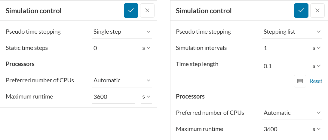
- Pseudo-time stepping: Select between solving a single time step or a list of time steps.
- Single Step: A single load case is run.
- Stepping list: Allows to run a list of load cases, ordered by the pseudo-time variable.
- Static time steps: Selects which time step is run if Single Step is selected. Default to zero if not using multiple time steps.
- Simulation intervals/Time step length: Allows to program which load cases will be run, in this way:
- Simulation intervals: End value of the pseudo-time variable. Default value is 1.
- Time step length: Increment value of the pseudo-time variable. Default value is 0.1, which combined with the default interval of 1, will lead to the execution of 10 cases, with time values of 0.1, 0.2, 0.3, and so on up to 1.
Nonlinear Static and Dynamic Analysis
In a nonlinear static or dynamic analysis, one or more properties are allowed to vary with time, such as material properties (plasticity or hyperelasticity), load curves, and nonlinearities such as physical contact. Thus, it is necessary to control the time integration values, such as the end time and time step length. For this purpose, two main strategies exist: manual or automatic (adaptive) time step definitions.
Manual Time Step
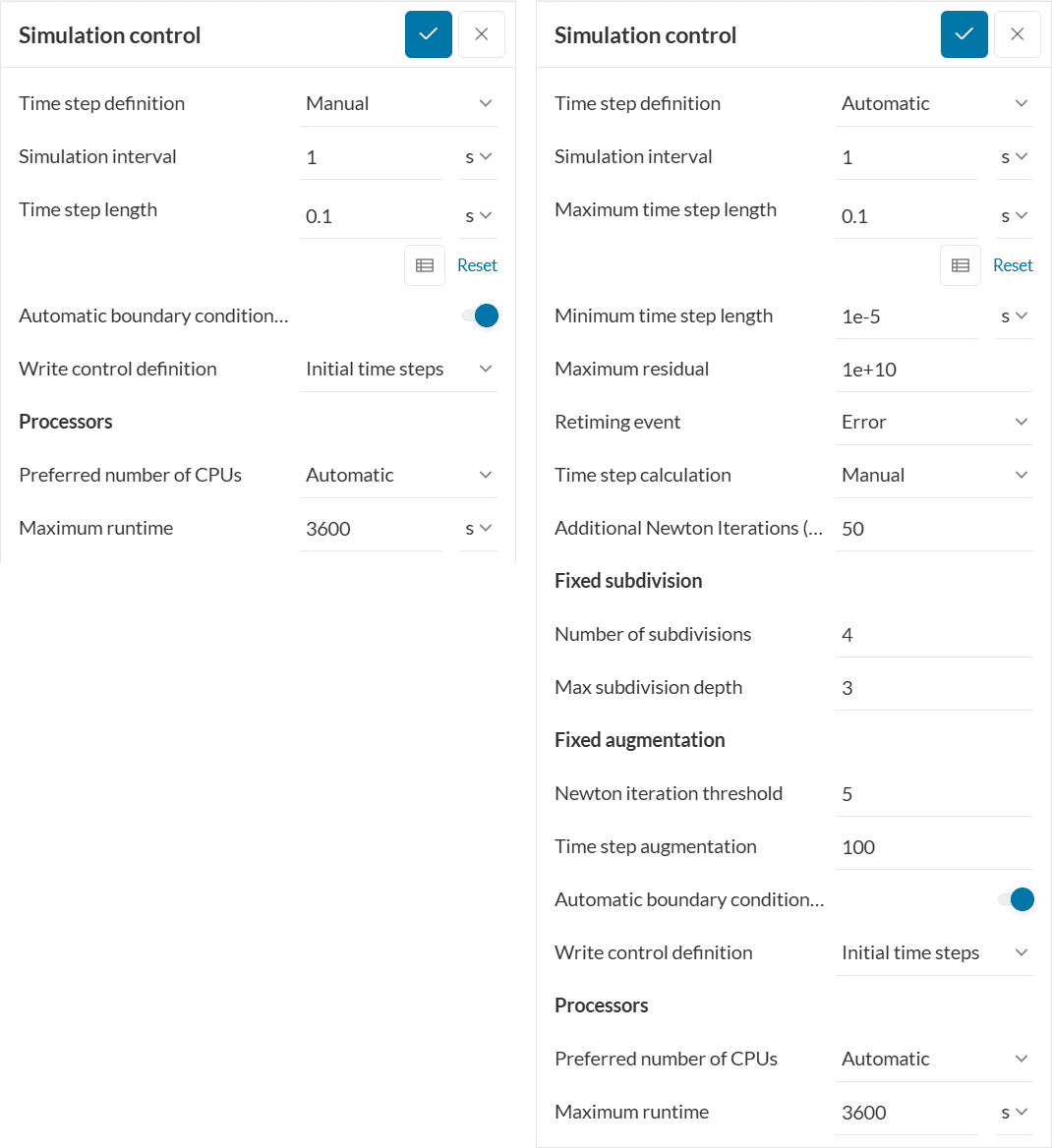
With this option, the list of integration steps is fixed and predefined by the user. It can lead to convergence problems if the time step is too large with respect to the change in the computed results. The following parameters are available:
- Simulation Interval: End time for the simulation.
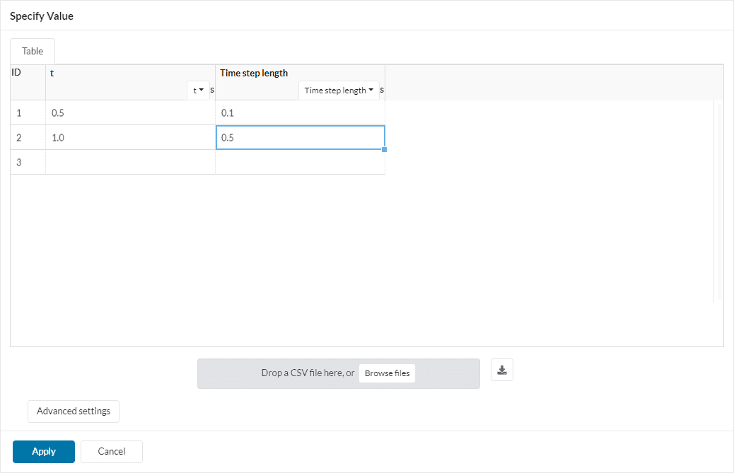
- Time step length: The interval between each subsequent integration time. A single value can be specified for the whole simulation interval, or multiple values per interval can also be specified. For this purpose, use the ‘variable’ button to open the ‘Specify Value’ window (see the picture). Here, a table is inputted with each row defining one interval:
- t: ‘Up to time’, specifies the end time for each interval.
- Time step length: specifies the time step for each interval.
- Automatic boundary condition ramping: In nonlinear static simulations, loads and displacements are typically ramped up with table or formula definitions to help with convergence.
In case the setup only contains constant loads and/or displacements, then the Automatic boundary condition ramping option causes the following constant definitions to be automatically ramped linearly throughout the nonlinear static run: fixed value, remote displacement, rotating motion, centrifugal force, follower pressure, force, nodal load, pressure, remote force, surface load, volume load, and gravity.
Furthermore, in case a material has been defined with any creep models enabled, automatic ramping will not be applied.
Did you know?
The manual time step length assignment requires extra care. Please check this article to learn more about how to determine the manual time step length.
Automatic (Adaptive) Time Step
With this option, the adaptive time step scheme can be used. The strategy consists of subdividing the current time step into smaller time steps each time an error event occurs. This way, most convergence problems are overcome by using smaller time steps. The available parameters are:
- Simulation interval: The end time of the simulation.
- Maximum time step length: Initial time step intervals used for the simulation, before any step cutting is performed. Here, the same scheme as in a manual time step strategy is used, so please refer to that section above for details.
- Minimum time step length: The minimum allowed time step interval after any subdivision. If the threshold is crossed after a step cutting, an ‘Automatic timestepping lead to a timestep below the minimum threshold‘ error is thrown.
- Maximum residual: Maximum allowed residual from a Newton iteration before a divergence error happens.
- Retiming event: Select which event triggers a time step subdivision. Possible choices and its trigger events are:
- Error: divergence or matrix singularity
- Collision: change in a physical contact state from open to closed
- Field change: a specific threshold value for change in a given field can be chosen. For example, the X component of displacement being higher than 0.1 m.
- Non-monotonous residual: the residual has not been reduced for the past three iterations. This allows saving computing time by cutting the newton iterations early.
- Time step calculation: Select how the smaller time step is computed. The available strategies depend on the selected retiming event:
- Manual: Available for error, collision, and non-monotonous residual events. The current time step length is subdivided into equal number of steps, according to the given parameters under Fixed subdivision. Also, under a given circumstance, the time step length can be augmented back to save on computing time, according to the given parameters under Fixed augmentation.
- Additional percentage of Newton iterations: The solver is allowed to keep iterating at the current time if the residual is monotonically decreasing and expected to reach the threshold within the given number of additional iterations. The allowed number of additional iterations is expressed as a percentage of the maximum newton iterations specified in Numerics.
- Number of subdivisions: Number of equal divisions of the current time step.
- Max subdivision depth: Maximum number of times the subdivision will be carried out.
- Newton iteration threshold: Criteria to trigger the augmentation. If on one time integration step convergence is achieved in a number of Newton iterations lower than this parameter, the time step will be augmented.
- Time step augmentation: Percentage of time step augmentation, e.g., for the default value of 100%, the time step will be doubled.
- Newton iterations target: Available for error, collision, and non-monotonous residual events. The solver estimates the time step length necessary to achieve the target Value of newton iterations before convergence, based on the residual change of the last time step.
- Field change target: Available only for field change event. The solver estimates the time step length necessary to achieve the target field change Value, based on the field change of the last time step.
- Mixed: available only for field change event. The subdivision is performed with a fixed subdivision just like in the manual strategy. The augmented time step is estimated by the solver to meet the Field change target.
- Manual: Available for error, collision, and non-monotonous residual events. The current time step length is subdivided into equal number of steps, according to the given parameters under Fixed subdivision. Also, under a given circumstance, the time step length can be augmented back to save on computing time, according to the given parameters under Fixed augmentation.
- Automatic boundary condition ramping: In nonlinear static simulations, a good practice is to ramp up displacements and loads with a table or formula definitions, as it helps with simulation convergence.
In case the setup only contains constant loads and/or displacements, then the Automatic boundary condition ramping option causes the following constant definitions to be automatically ramped linearly throughout the nonlinear static run: fixed value, remote displacement, rotating motion, centrifugal force, follower pressure, force, nodal load, pressure, remote force, surface load, volume load, and gravity.
Furthermore, in case a material has been defined with any creep model enabled, automatic ramping will not be applied. - Write control definition: Select in which time steps the output fields are written to the results database. Available options are:
- Write interval: The output times are selected by skipping a fixed number of time steps. The number of steps to skip is given by the Write interval value.
- All computed: All the computed time steps are written, including the ones generated due to subdivisions.
- Initial time steps: The output is written on the time steps specified under Maximum time step length.
- User defined: The user can define the time steps to write the output, using the same scheme from the Manual time step strategy.
Heat Transfer
In a heat transfer analysis, linear on nonlinear, the steady state condition is assumed, thus there are no time step computation controls.
Nonlinear Thermal Analysis
The only allowed non-linearity in a thermal analysis is temperature dependency of the boundary conditions and material properties.
Thermomechanical
Thermomechanical analysis is a succession of heat transfer analysis and structural analysis, where the temperature field is computed first and then converted to thermal expansion strains for the structural analysis. The available simulation controls depend on the selection of structural parameters under global settings like linear static, nonlinear static or dynamic, for which detailed explanations are already given above.
Frequency Analysis
Three options are available for the control of natural frequencies to be computed, selecting how they are searched: First modes, Center frequency, and Frequency range.

- Eigenfrequency Scope:
- First modes: The first Number of modes will be searched and computed, in the order of low to high frequency.
- Center frequency: A certain Number of modes will be determined around a center frequency of interest.
- Frequency range: All the modes within the range of frequencies will be searched and computed. The frequency range is specified by a Start frequency and an End frequency.
Harmonic
Two options are available for the control of the excitation frequency to be considered on the computation: Single frequency and Frequency list.
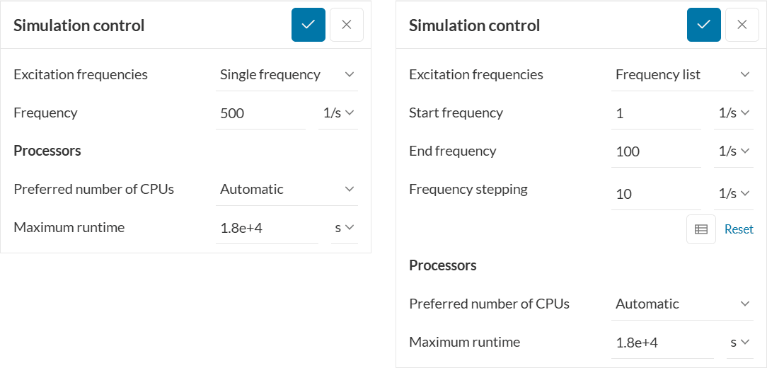
- Excitation frequencies:
- Single frequency: The one excitation Frequency value that will be considered in the harmonic computation.
- Frequency list: A range of frequencies between Start frequency and End frequency, with a step given by Frequency stepping. If a non-regular stepping is desired, a table input can be used to specify the list of frequency steps:
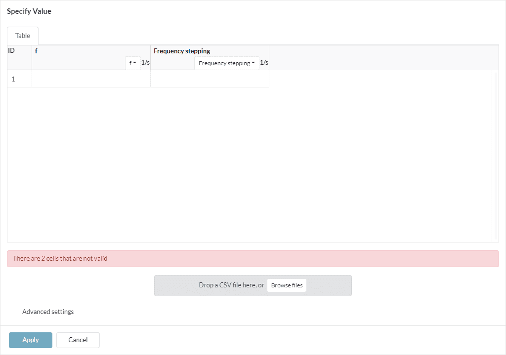
If using the table option, each successive row defines a frequency sub-range, with the end frequency of the interval given by the f column, and the sub-stepping given by the Frequency stepping column.
Last updated: July 10th, 2025
Did this article solve your issue?
How can we do better?
We appreciate and value your feedback.


