Linear Contacts
Two bodies are said to be in contact when they share at least one common boundary and the boundaries are constrained by a relation (i.e. no relative movement).
In the case of structural simulations, the multiple parts in an assembly are discretized into multiple non-conforming mesh parts, i.e. the single bodies are meshed separately by the meshing algorithm and do not share the nodes lying on their contacting entities, thus they are not connected. In order to ensure the mechanical interaction between the parts, they have to be related via contact constraints, which create the proper coupling between the degrees of freedom.
Automatic Contact Detection
In order to guarantee that the simulated domain is properly constrained, all contacts in the system will be detected automatically whenever a new CAD assembly is assigned to a simulation (this also includes simulation creation). By default, all contacts in the assembly will be created as Bonded contacts, which can later be edited by the user.
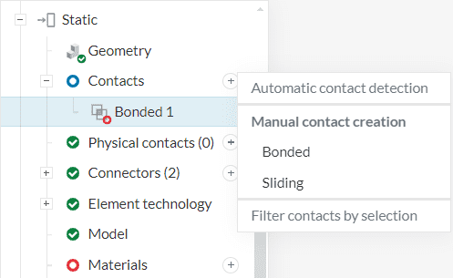
Contact detection can also be triggered manually via the context menu of the Contacts node in the simulation tree by clicking on the ‘+ button’:
While contacts are being detected, the Contacts in the simulation tree is locked. The time required for contact detection depends on the size and complexity of the geometry and can take between a few seconds to a few minutes. A loading indicator on the contact tree node signals that contact detection is ongoing.
Bulk Selection
Depending on the size and complexity of an assembly, the number of contacts created can become quite large.
An easy way to edit multiple contacts at once is via bulk selection. The bulk selection panel exposes all contact options besides assignments to the user for editing.
Contacts can be selected in bulk via CTRL + Click and/or SHIFT + Click in the contact list or via the filter contacts by selection option in the viewer context menu. The Filter contacts by selection option returns contacts based on the current selection.
The following selection modes are possible:
- One volume selected: All contacts that contain at least 1 face on the selected volume will be selected.
- Two or more volumes selected: All contacts that contain at least one face on at least two of the selected volumes will be selected.
- One or multiple faces on one body selected: All contacts that contain at least one of the selected faces will be selected.
- Multiple faces across more than one volume selected: All contacts that contain at least one of the selected faces from at least two of the volumes will be selected.
Linear Contact Types
Currently, there are two types of linear contact constraints available:
- Bonded contact
- Sliding contact
Bonded Contact
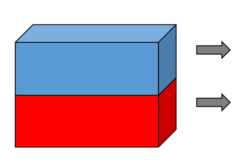
The bonded contact is a type of contact that allows no relative displacement between two connected solid bodies. This type of contact constraint is used to glue together different parts of an assembly.
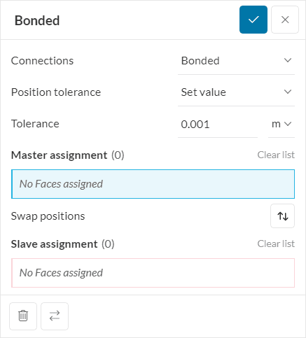
You can assign faces or sets of faces that should be tied together via the assignment box under Pick Faces. For numerical purposes, you have to choose one of these selections as master and the other one as slave. During the calculation, the degrees of freedom of slave nodes are constrained to the master surface.
When running contact analyses, the position tolerance can be set manually or turned off. The position tolerance defines the distance between any slave node and the closest point to the nearest master face.
When tolerance is turned on, only those slave nodes that are are within the defined range from a master face will be constrained. When the tolerance is set to off, all slave nodes will be tied to the master surface absolutely. Therefore, if a larger face is used as a master, one slave node will be tied to multiple master nodes leading to artificial stiffness in the slave surface.
Note
If a larger surface (or surface with higher mesh density) is chosen as slave, the computation time will increase significantly and it might also result in a wrong solution, especially when no specific tolerance criteria is provided.
Sliding Contact
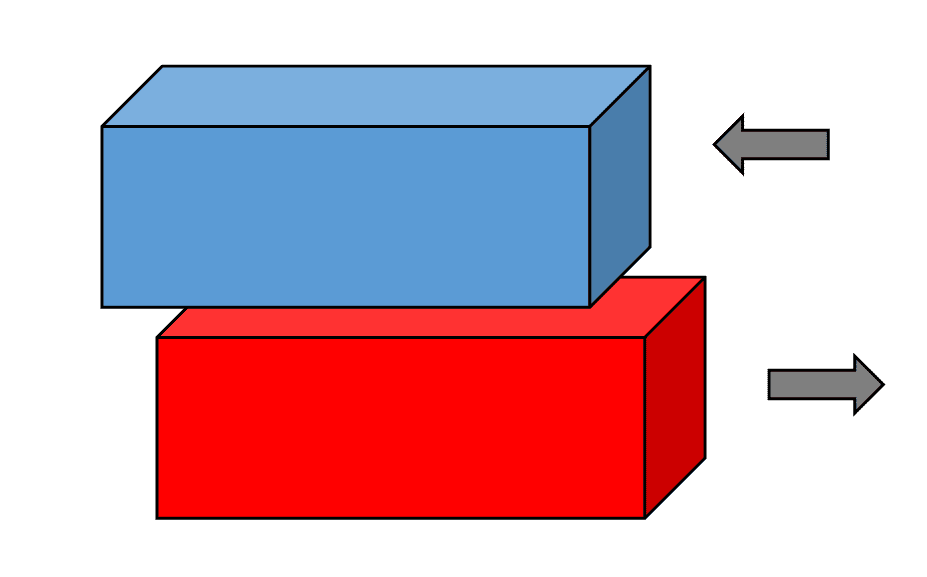
The sliding linear contact allows for displacement tangential to the contact surface but no relative movement along the normal direction. This type of contact constraint is used to simulate sliding movement in the assembly for linear simulations. The two surfaces that are in contact are classified as master and slave. Every node in the slave surface (slave node) is tied to a node in the master surface (master node) by a constraint.
You can assign faces or face sets that should be tied together via the assignment boxes under Pick Faces. For numerical purposes, you have to choose one of these selections as master and the other one as slave. During the calculation, the degrees of freedom of slave nodes are constrained to the master surface while only allowing tangential movement.
Important
The sliding contact is a linear contact constraint which is intended for planar sliding interfaces. Therefore, no large displacements and rotations are allowed in the proximity of a sliding contact. In other words, this constraint is not suitable for nonlinear simulations.
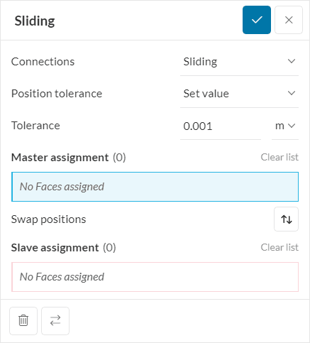
Master and Slave Assignments
When setting up linear contacts, master and slave assignments must be defined in the setup window. If the contact faces are different in size, as a rule of thumb the smaller faces should be set as slave faces.
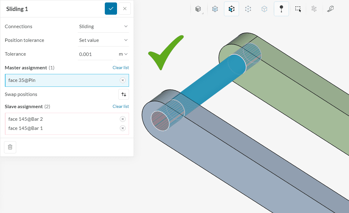
In the example below, a sliding contact between a pin and two bars is defined according to best practices. Since the pin is larger than the holes in the bars, the pin is correctly defined as the master assignment:
In the next example, the bonded contact is not defined according to best practices. Since the tank face is much larger than the leg faces, the tank should have been the master assignment.
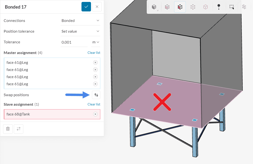
In the image above, a quick way to invert the master and slave assignments is to click on the Swap positions icon, indicated by the blue arrow.
Important
The importance of slave and master assignments comes from the fact that all nodes of the slave will be bound to the nearest master element within the tolerance.
If the larger side is selected as slave this often leads to over-stiffening of the slave surface.
Last updated: October 1st, 2024
Did this article solve your issue?
How can we do better?
We appreciate and value your feedback.


