Custom Boundary Condition
The Custom boundary condition gives users the freedom to define a customized boundary condition that fulfills the requirements for a particular problem. This is only recommended for advanced users if there is a need to implement a boundary condition outside of the standard boundary options. The custom boundary conditions are only available for fluid flow simulations.
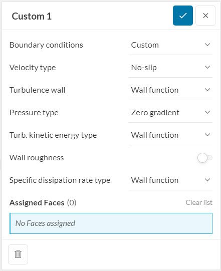
For the custom boundary condition, the user must specify first the types, and then the values of all the flow variables for a particular face/surface. All basic and advanced boundary condition types based on the OPENFOAM® code are available for the relevant flow variables.
Important
Care must be taken by the user to make sure that the model is not over or under-defined, and that the selections are not contradicting, or that they are logically correct in terms of the boundary conditions. No guarantees for stability, convergence, or validity are provided in this case.
Boundary Types and Flow Variables
Based on the selected analysis type, the custom boundary must be defined according to the available boundary types and flow variables that are further detailed below:
- Velocity type \([U]\): Settings to how the velocity is calculated or defined by the user on the boundary.
- Pressure type\([p]\): Settings to how the pressure is calculated or defined by the user on the boundary.
- Temperature type\([T]\): Settings to how the temperature is calculated or defined by the user on the boundary.
- Turbulent Kinetic Energy Type\([k]\): Settings to how the turbulent kinetic energy is calculated or defined by the user on the boundary.
- Specific Dissipation Rate Type\([\omega]\): Settings to how the specific turbulent dissipation rate is calculated or defined by the user on the boundary.
- Turbulence Wall: Settings to which approach to use for the wall treatment.
- Wall roughness: Settings to to model wall roughness. The user can toggle on or off this setting in order to include the roughness of the surface.
- Roughness height: A representative distance to the wall.
- Roughness constant: A parameter that measures how uniform the roughness is.
- Prandtl number \([Pr]\): It’s a dimensionless number approximating the ratio of momentum diffusivity (kinematic viscosity) to thermal diffusivity.
- Turbulent dynamic viscosity \([μ_t]\): It is required to account for the transport and dissipation effects lost in averaging the turbulence.
- Turbulent thermal diffusivity \([α_t]\): Defines the behavior of thermal diffusion at the face/surface.
- Phase fraction \([\alpha]\): Settings on the fraction between the phases in a multiphase simulation.
- Eddy viscosity \([ν_t]\) : It models the transport and dissipation of energy that was neglected as a result of turbulence modeling.
- NuTilda \([\tilde{\nu} ]\): A Spalart-Allmaras variable that is a function of eddy viscosity.
- Turbulence dissipation \([\epsilon]\): Defines the dissipation rate of the turbulent kinetic energy when using a k-epsilon turbulence model.
Condition Types
Each boundary setting, such as Velocity type, Pressure type, etc. should be defined by selecting one of the condition types. Each setting can either be calculated by the solver using related equations or be defined manually by the user. Several conditions based on the OPENFOAM® code are provided for the boundary settings while defining custom boundaries.
Some of these conditions are applicable for all boundary settings while some of them are limited to a few. Conditions that are applicable for all boundary settings are listed under the General section below. Other conditions that are applicable to specific boundary settings are listed accordingly.
General
Condition types listed in this section are applicable for all boundary type settings.
Symmetry
Symmetry conditions can be used in several types of simulations to take advantage of the symmetric behavior of the application. This condition is applied to planar patches to represent symmetry conditions. Velocity, pressure, temperature, turbulence variables, and phase fraction boundary settings are applicable for this condition type.
Fixed Value
Fixed value, also known as Dirichlet type, is a boundary type where the value at the boundary face is defined by the user.
$$\phi_f = \phi_{ref}$$
where \(\phi_f\) is the value at the face,
\(\phi_{ref}\) is the reference value that should be defined by the user.
Velocity, pressure, temperature, turbulence variables, and phase fraction settings are applicable for this condition type.
Fixed Gradient
Fixed gradient, also known as Neumann type, is a boundary type in which the gradient normal to the boundary face is specified by the user. Values at the boundary face are calculated according to:
$$\phi_f = \phi_c +\Delta \nabla \phi_{ref}$$
where \(\phi_f\) is the value at the face,
\(\phi_c\) is the value in the cell adjacent to the face,
\(\nabla \phi_{ref}\) is the reference gradient that should be defined by the user,
\(\Delta\) is the distance from the cell center to the face.
Velocity, pressure, temperature, turbulence variables, and phase fraction settings, for e.g. in multiphase simulations, are applicable for this condition type.
Zero Gradient
Zero gradient type is a derived condition type based on fixed gradient where the values at the boundary are equated to the internal field value. Gradients that are used to calculate face values based on internal values are simply equated to zero.
$$\frac{\delta}{\delta n} \phi = 0$$
This condition can be used for velocity, pressure, temperature, turbulence variables, and phase fraction in multiphase simulations as well.
Inlet-Outlet
This boundary type is usually used for outlet conditions where there are possible reverse flows. Therefore an inflow value should be specified by the user to handle reverse flows. This condition type switches between two operations that are: either a fixed value defined by the user for the flows entering the domain, or a zero-gradient condition for the flows leaving the domain. This condition can be used for velocity, pressure, temperature, turbulence variables, and phase fraction in multiphase simulations as well.
Advective
Users can define this boundary type to let sound waves exit the domain without being reflected near the outlet boundaries. Reflection near the outlets may have a significant effect when the flow is compressible. Hence, this boundary type is only available in the Compressible simulation type.
This outflow condition is applied to the boundary by equating the material derivative of the variable of interest to zero. Additionally, the boundary can be relaxed by enabling Relax boundary toggle. However, this will require two additional inputs: Far field value and Relaxation length scale. This condition type can be used for velocity and pressure.
Radiative Behaviour
Once the radiation is enabled, users are obliged to define the radiative behavior of all boundaries including custom ones. In SimScale platform, radiative behavior can be set to transparent or opaque, and each selection requires a different input type.
Velocity
Condition types listed in this section are only applicable to velocity type boundary settings.
Mean Value
This condition type is mostly used when it’s not clear whether the flow that passes through the boundary face is distributed uniformly, or not. The average value of the applicable flow variables will be equated to a value defined by the user. Unlike the fixed value condition type, not every cell face on the boundary will have the same value. This condition is usually applicable for outlet boundaries where the flow behavior is not exactly clear.
Flow Rate
The flow rate type is a wrapper around the fixed value type, and sets the velocity to a user-defined profile. This condition calculates velocity at the boundary face based on the provided flow rate.
Mean Flow Rate
This type should only be used for inlet conditions when the exact distribution of the flow variables passing through the boundary face is not clear. Similar to the mean value boundary type, an average value of the flow rate will be equated to a value defined by the user.
Freestream
Freestream condition type should be used when the boundaries are far from the objects. This condition is derived from the Inlet-Outlet condition type and applies a fixed value velocity for the inlet and a zero gradient condition at the faces where flow is leaving the domain based on the patch normal velocity. (Unlike the inlet-outlet condition type which blend between fixed value and zero gradient based on the flux) There is no need to assign seperate boundary conditions for the inlet and outlet. This type is only available for velocity and pressure type settings since it’s exactly the same with inlet-outlet condition for other variables.
Pressure Inlet Velocity
This condition type is used to calculate the velocity on a boundary face based on the pressure specified on the same boundary face by the user. Entering velocity is calculated based on the flux with a normal direction to the boundary faces. This condition type is only available for velocity type setting, but it’s constrained by the pressure type setting while defining custom boundary conditions. Users are encouraged to define Pressure Inlet-Outlet Velocity type instead of Pressure Inlet Velocity if there is a possible reverse flow on the boundary face.
Pressure Inlet-Outlet Velocity
Pressure Inlet-Outlet Velocity type should be used when there is a need to calculate velocity on a boundary face based on the pressure values specified by the user, and there is a possible reverse flow. Similar to Inlet-Outlet condition, zero gradient is applied for the flows leaving the domain. The velocity is obtained based on the flux with a normal direction to the boundary faces. This condition type is only available for velocity type settings. However, it’s constrained with the pressure type setting while defining custom boundary conditions.
Wall
Users are able to define wall boundary conditions with several characteristics by using custom boundary conditions. Wall boundary can be customized by selecting one of the wall types which are: no-slip, slip, moving wall and rotating wall. These conditions are only available for velocity type settings.
Pressure
Condition types listed in this section are only applicable to pressure type boundary settings.
Mean Value
This condition type is mostly used when it’s not clear whether the flow that passes through the boundary face is distributed uniformly, or not. The average value of the applicable flow variables will be equated to a value defined by the user. Unlike the fixed value condition type, not every cell face on the boundary will have the same value. This condition is usually applicable for outlet boundaries where the flow behavior is not exactly clear.
Total Pressure
This is a derived condition type by using the fixed value condition, and it’s used to set the static pressure on the boundary face by using the user-defined total pressure value. Static pressure, and velocity value at the face are adjusted until they reach a converged state.
Fixed Flux
Fixed flux pressure condition type is only available for pressure type settings. It can be used to set the pressure gradient according to the flux on the boundary defined by condition types for velocity. This type is mostly used when body forces such as gravity are present in the solution. Hence, it’s only available in simulations that can model gravity.
Fan Pressure
Fan pressure condition type sets the static pressure \(P_s\) at the boundary face based on the user-defined ambient total pressure \(P_t\), and fan pressure curve \(P_{Fan}\).
$$P_s = P_t – P_{Fan}$$
Fan pressure values should be defined by the user as a function of volumetric flow rate by using the tables. This condition type can either push air into the fluid domain or create suction to extract air from the fluid region.
Temperature
Condition types listed in this section are only applicable for temperature type boundary settings.
External Wall Heat Flux
External wall heat flux applies a heat flux condition to the temperature on an external wall in one of two modes. These two modes are Fixed heat flux and Derived heat flux. One of the modes should be chosen depending on the application. This condition is mostly used for walls, and is only available for temperature type boundary settings. External wall heat flux condition type can be used for surfaces when corresponding heat flux values can be specified such as external walls of buildings, windows, etc.
Adiabatic
As the name suggests, this is used for walls that have no heat transfer through, and the temperature has zero gradients. Adiabatic condition type is useful to model perfect insulators.
Total Temperature
This is a derived condition type by using the fixed value condition, and it’s used to set the static temperature on the boundary face by using the user-defined total temperature value. It’s mostly used for compressible flow simulations, and it requires an additional input parameter: the ratio of specific heats.
Turbulent Heat Flux
Turbulent heat flux provides a fixed heat constraint on temperature. Temperature gradient through an input heat source can be specified either by defining an absolute power or heat flux. This condition type is derived by using a fixed gradient condition type. Turbulent heat flux conditions can be preferred to model the power sources in simulations such as: humans, computers, etc.
Wall Heat Transfer
This condition type provides an enthalpy condition for wall heat transfer. It requires a surface temperature and an additional thermal input parameter: thermal diffusivity which defines the behavior of thermal diffusion at the face/surface.
Turbulence
Condition types listed in this section are only applicable for turbulent kinetic energy, and specific dissipation rate type boundary settings.
Wall Function
This condition type should be used mostly for walls, and it provides appropriate functions to model the velocity profile when it’s used for turbulence wall boundary setting. Wall functions can also be used to calculate turbulent kinetic energy, and specific dissipation rate by providing wall functions at the boundary face.
Full Resolution
The Full resolution condition type can be used for cases where there is a need to resolve the flow profile completely instead of modeling. It can be used for the Turbulence Wall boundary setting to fully resolve the velocity profile near the wall. Similar to the wall function condition type, this condition can also be used to calculate turbulent kinetic energy production and specific dissipation rate. Users should be aware that using the full resolution condition type requires denser mesh elements near the boundary face which will significantly affect the computation time and resources.
Intensity Inlet
This condition type is used to define the turbulent kinetic energy type at the boundary faces. Turbulence intensity represents a standard deviation between the velocity fluctuation and the average velocity of the flow. By using the intensity value, specified by the user, turbulent kinetic energy is calculated. Please note that the turbulence intensity is given in absolute values, therefore, defining a turbulence intensity of 0.01 is equivalent to 1%.
Availability in Simulations
Custom boundary conditions can be used to simulate accurate physics that are applicable for each simulation type. However, due to the difference in mathematical characteristics of governing equations in each simulation type, there isn’t a common solver that can accurately work on all of them. Each simulation requires unique inputs for the solution, so available boundary conditions in each simulation will be different as well. The custom boundary conditions in SimScale are only available for fluid flow analyses.
Incompressible
A. Atmospheric Boundary Layer
One of the most common application in incompressible simulations when custom boundary conditions are used is atmospheric boundary layers. Users can define custom inlet boundary conditions by using equations for atmospheric boundary layers. Those interested are encouraged to follow this advanced tutorial.
B. Still Ambient Air
Another common workflow that requires custom boundary conditions, is when the properties at the atmospheric boundaries are not known. This can be caused by the interaction between the geometry and flow, or advanced concepts such as rotating zones and momentum sources. In this drone simulation, a custom boundary condition for the faces open to the atmosphere is defined with the pressure inlet-outlet velocity condition type. This setting allows the solver to compute the flow variables whether there’s an inflow or outflow.
Compressible
In compressible simulations, temperature values are also important, since the equation of state and energy equations are solved. Hence, while setting up custom boundary conditions for a compressible simulation, temperature type boundary setting along with all others will be available for users to specify.
A. Increasing the outlet stability
Custom boundary conditions can be used in compressible simulations for purposes also applicable to all other simulation types. In this validation case, a custom boundary condition is applied at the inlet face to specify a turbulent kinetic energy production value and specific dissipation rate using the fixed value condition. In order to enhance stability, an outlet type boundary is generated by using custom boundary conditions as well. Zero gradient for velocity type and a fixed value for pressure type are defined such that the combination of the inlet and outlet boundaries provides stable solutions with better convergence.
Convective Heat Transfer
All boundary type settings while defining custom boundary conditions are available for convective heat transfer simulations, except for multiphase parameters.
A. Fan Condition
Custom boundary conditions can be used in convective heat transfer simulations to enhance stable inlet and outlet combinations, to define outlets where the flow behavior is not very clear, to specify custom external fan boundaries, etc. In this particular study, a transient convective heat transfer is performed with external fan boundaries. To create the fan boundary condition, pressure inlet-outlet velocity condition type for velocity type setting, fan pressure for pressure type setting, and adiabatic condition type for temperature type setting are used.
B. Simulating a Server Rack
In this validation case on airflow in a data center, custom boundary conditions are used to model the hot sides of the racks in the data center based on the flow rate through the server rack, the temperature at the cold side, and the heat dissipation. . Velocity, temperature, turbulent kinetic energy, and specific dissipation rate are specified on the boundary faces.
Multiphase
While defining a custom boundary condition in multiphase simulations, an additional boundary setting is required: phase fraction. Users need to either define a general condition for the phase fraction such as a fixed value or a contact angle.
The contact angle boundary condition is used when there is a need to set the contact angle at the walls. Curvature in the cells closest to walls is calculated by using this value. Therefore, it’s needed for a proper calculation of surface tension in those cells. In other words, the contact angle is used to adjust the surface normal vector to the interface in cells near the wall.
Two options are available to define the contact angle on the walls. The static contact angle can be used when the amount of change in advancing and receding contact angles is not significant for the application. For simple cases where the surface tension effects can be ignored between the wall and interface, e.g. water moving inside a large tank, a static contact angle of 90 degrees can be defined. This can also be achieved by defining a zero gradient condition type for the phase fraction setting.
A dynamic contact angle should be used when the amount of change between advancing and receding angles are significant. An example is water droplets on tilted surfaces. An experimental investigation is needed to decide whether the difference in advancing and receding contact angles is significant or not, as well as to obtain these contact angles in case of dynamic contacts are needed.
Last updated: April 2nd, 2025
Did this article solve your issue?
How can we do better?
We appreciate and value your feedback.


