Thermophysical Fluid Models
Thermophysical models define how the energy, heat, and physical properties of the fluid are calculated. These variables are then determined based on the analysis type and the selected models. The models are relations of a pressure-temperature equation system using which the required fluid properties and variables are then calculated.\(^1\)
Thermophysical fluid models can be selected under Materials after a material has been selected from the library. They are only available for compressible flow simulations. Hence, convective, conjugate heat transfer (both solvers), and Multi-purpose simulations need to have compressibility toggled on.
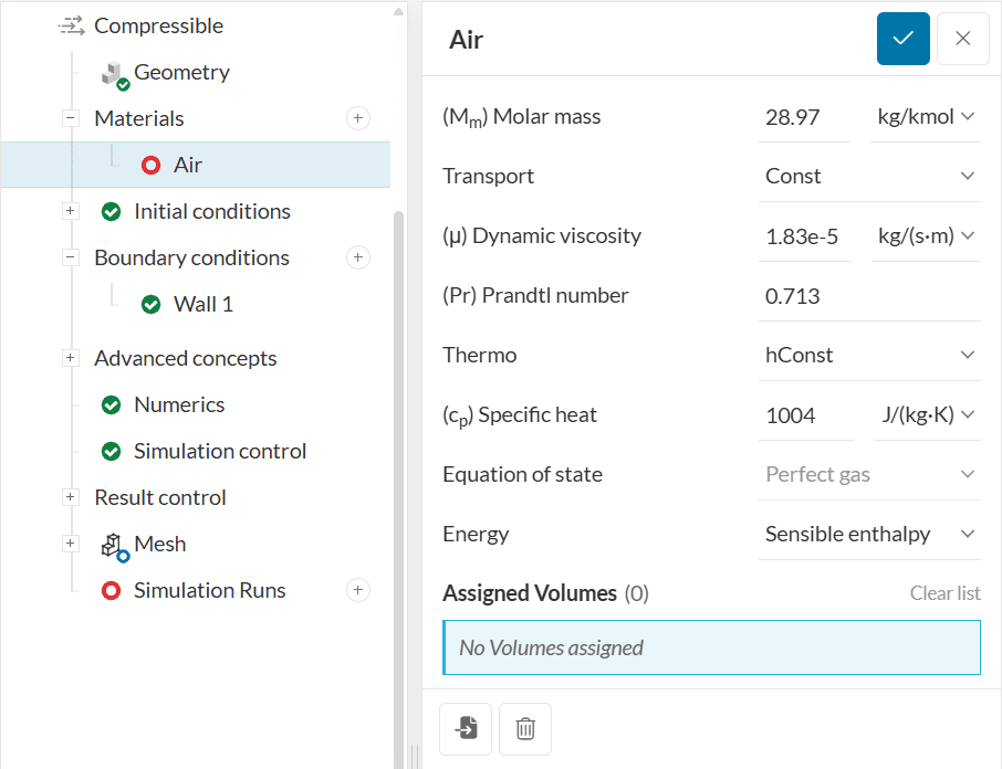
These settings are briefly described as follows:
1. Fluid Type
This setting is specific to multi-purpose compressible simulations, allowing the user to define whether a fluid is a Liquid or a Gas.
2. Molar Mass
Molar mass \((M_m)\) represents the molecular weight of the component per mole in units of \(kg/kmol\) or \(lb/kmol\) and is dependent on the molecular structure of the fluid material.
3. Transport Model
The transport model relates to the calculation of the transport variables dynamic viscosity \((\mu)\), thermal conductivity \((\kappa)\), and thermal diffusivity \((\alpha)\) for energy and enthalpy equations.\(^1\) Depending on the analysis type, the following types of transport models are available:
Const (Constant parameters)
The Const type will assume a constant dynamic viscosity, \(\mu\) and Prandtl number, \(P_{r}= c_{p}\ \mu / \kappa\) . These parameters are then specified in the panel.
Sutherland
For the Sutherland type, the dynamic viscosity \((\mu)\) is not constant, and changes with temperature \((T)\). The dynamic viscosity is then calculated as a function of temperature given by the relation:
$$ \mu = \mu_0 \frac{T_0 + T_s}{T + T_s} \left(\frac{T}{T_0}\right)^{3/2} \tag{1}$$
where:
- \(T_s\) is the Sutherland’s temperature with SI units \(K\)
- \(T_0\) is reference temperature in \(K\)
- \(\mu_0\) is the reference viscosity (at the reference temperature), in SI units of \(\frac{kg}{s.m}\)
- \(T\) is the static temperature of the fluid in \(K\)
- \(\mu\) is the viscosity of the fluid in SI units of \(\frac{kg}{s.m}\), calculated at the temperature \(T\)
Referring back to Figure 1 in this documentation page, the user provides \(\mu_0\), \(T_0\), and \(T_s\) in the simulation set up. The Sutherland’s temperature (sometimes referred to Sutherland’s Constant) can be found online\(^2\) for a variety of fluids.
4. Thermo Models
Thermo models are used to calculate the specific heat at constant pressure \((c_{p})\) for the fluid, from which the other properties are then derived. The following methods are available for the evaluation of \(c_{p}\).
hConst
This option assumes a constant value for specific heat at constant pressure, \(c_{p}\) and the heat of fusion, \(H_{f}\).
eConst
This option does not assume a constant value for \(c_{p}\). Rather, it assumes the specific heat at constant volume, \(c_{v}\) and the heat of fusion, \(H_{f}\) to be constant.
5. Equation of State
An equation of state is a thermodynamic relation describing the interconnection between various macroscopic properties of a fluid. In OpenFoam solver, it describes the relation between density \((\rho)\) of a fluid and the fluid pressure \((P)\) and temperature \((T)\).\(^1\)
Based on the thermophysical model type, the following equations of state can be used:
| Equation of State | Solvers (With Compressibility Enabled) |
| Rho Const | Convective heat transfer, conjugate heat transfer, multi-purpose |
| Perfect Gas | Compressible, convective heat transfer, conjugate heat transfer, multi-purpose |
| Real Gas | Multi-purpose |
| Incompressible Perfect Gas | Convective heat transfer |
| Perfect Fluid | Convective heat transfer |
| Adiabatic Perfect Fluid | Convective heat transfer |
Rho Const
In this case, the fluid density \((\rho)\) is kept constant and does not change by pressure \((P)\) or temperature \((T)\)
$$ \rho = constant \tag{2}$$
The Rho Const model is available in convective heat transfer, conjugate heat transfer, and multi-purpose solvers.
Perfect Gas
For the case of perfect gas, the fluid is assumed to be an ideal gas and obey the ideal gas law, that is the equation of state as given by the following relation:
$$ \rho = P/(R_{specific}T) \qquad \tag{3}$$
where, \(P\) is the pressure, \(R_{specific}\) is the specific gas constant and \(T\) is the temperature.
Furthermore, the specific gas constant is given by the following equation:
$$ R_{specific} = R/M \qquad \tag{4}$$
where \(R\) is the universal gas constant, and \(M\) is the molar mass of the gas, defined under the Materials tab.
The Perfect Gas model is available in compressible, convective heat transfer, conjugate heat transfer, and multi-purpose solvers.
Real Gas
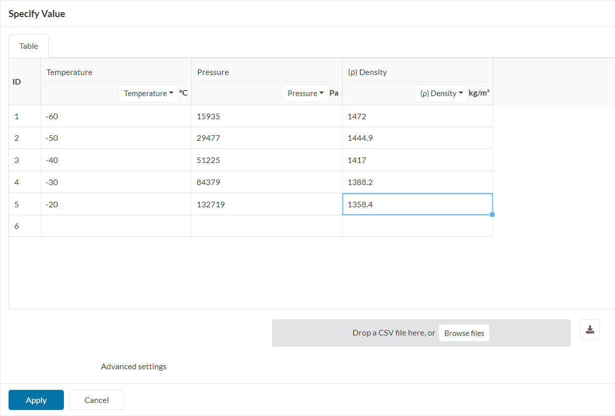
For all the cases where the fluid does not obey the ideal gas law, a generic real gas law definition can be used. This is a good option when the thermodynamic behavior of the fluid is known.
Users should be able to upload table input of thermodynamic properties like dynamic viscosity, density, and enthalpy as a function of temperature in a CSV format.
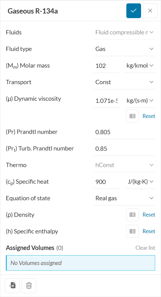
The real gas model is exclusive to the multi-purpose solver.
Incompressible Perfect Gas
In this case, the fluid is assumed a perfect gas that is only incompressible with respect to changes in pressure, \(P\). The equation of state is then given as:
$$ \rho = P_{ref}/(R_{specific}T) \qquad \tag{5}$$
where, \(P_{ref}\) is the reference pressure, \(R_{specific}\) is the specific gas constant and \(T\) is the temperature. The specific gas constant is calculated using equation 4. The incompressible perfect gas model is only available for convective heat transfer analyses with compressibility enabled.
Important
For incompressible perfect gas, the gas density \((\rho)\) can vary due to changes in temperature \((T)\) .
Perfect Fluid
In the perfect fluid case, the equation of state takes the form as given below:
$$ \rho=P/(RT) \ +\ \rho_{0} \qquad \tag{6}$$
where, \(\rho_{0}\) is the density at \(T = 0\). Then the density of the fluid can change both due to pressure and temperature. The perfect fluid model is exclusive to the convective heat transfer solver with compressibility enabled.
Important
This option is recommended to model natural convection in liquids, e.g., water, due to changes in temperature.
Adiabatic Perfect Fluid
The adiabatic perfect fluid model, available only for convective heat transfer studies with compressibility enabled, follows the following equation of state:
$$ \rho = \rho_0 \left(\frac{P+B}{P_0+B}\right)^{1/\gamma} \tag{7}$$
where \(P_0\) is the reference pressure, \(B\) is offset pressure for a stiffened fluid, and \(\gamma\) is the isentropic constant.
6. Energy
Under Energy, two options are available for the form of energy to be used in the solution. One is the sensible internal energy and the other is sensible enthalpy. The difference between absolute and sensible energy is the absence of heat of formation in the latter.
For example, absolute enthalpy \((h)\) is related to sensible enthalpy \((h_s)\) for a single specie as follows:
$$ h=h_s+c\ \Delta h_{f} \qquad \tag{8}$$
where, \(c\) is the molar fraction and \(\Delta h_{f}\) is the heat of formation.
Important
In most cases it is recommended to use sensible enthalpy, unless energy change due to reactions is expected.
References
Last updated: October 28th, 2025
Did this article solve your issue?
How can we do better?
We appreciate and value your feedback.


