Advanced Tutorial: Smoke Propagation From a Chimney
This article provides a step-by-step tutorial for smoke propagation in the open air, making use of the passive scalar transport formulation.
Overview
This smoke propagation simulation tutorial teaches how to:
- Set up and run a convective heat transfer simulation with passive species;
- Assign boundary conditions, material, and other properties to the simulation;
- Set up walls with a given wall roughness;
- Define an Atmospheric Boundary Layer (ABL) profile for the inlet;
- Mesh with the SimScale standard meshing algorithm;
We are following the typical SimScale workflow:
- Preparing the CAD model for the simulation.
- Setting up the simulation.
- Creating the mesh.
- Run the simulation and analyze the results.
1. Prepare the CAD Model and Select the Analysis Type
First of all click, the button below. It will copy the smoke propagation project containing the geometry into your workbench.
The following picture shows how the workbench looks after importing the project. You can use the translucent mode to view the whole geometry inside as well.
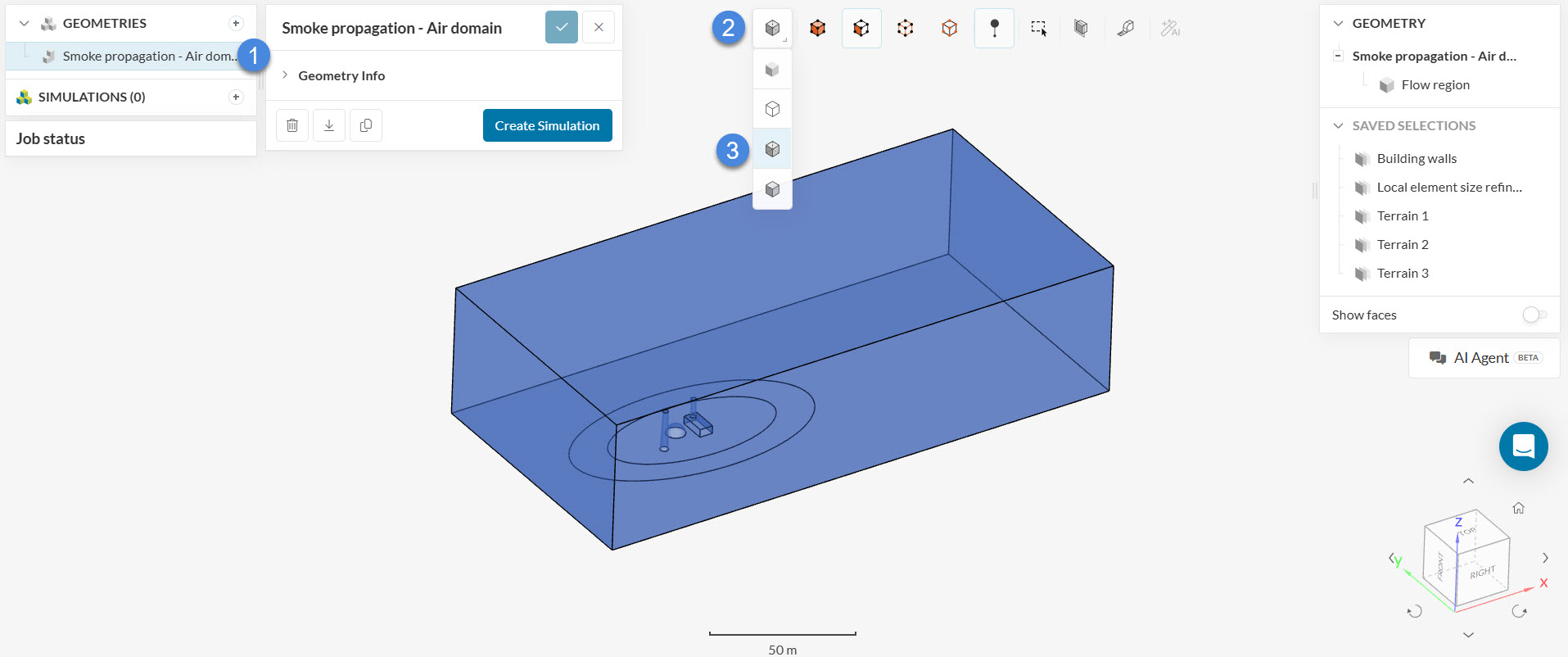
In this example, we want to have multiple faces on the ground to assign different terrain roughness. Therefore, we modeled the air domain in CAD software and split the ground surface.
The geometry is already prepared for the simulation stage. However, you can always make modifications to the model by using the CAD environment. To modify a CAD model, simply select the geometry from the list—the available CAD operations will then appear in the top toolbar. You can either work directly on the original model or create a duplicate and apply your changes to the copy.
Did you know?
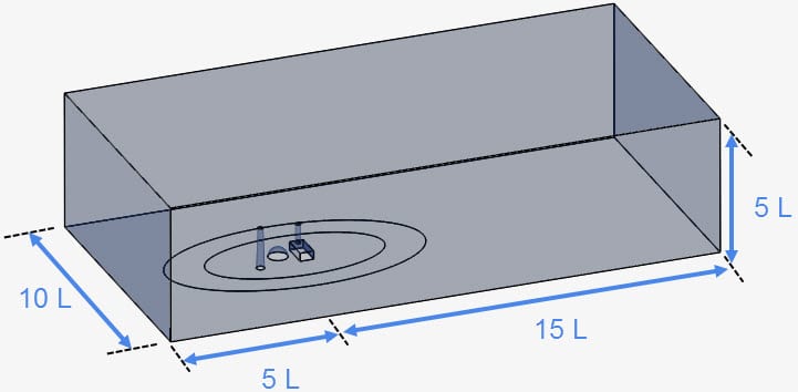
For simulations involving external flow, it’s important that the flow region is large. This is mostly necessary to avoid interferences from the boundaries. Furthermore, the domain should be longer downstream from the geometry, to capture the wake effects.
Assuming “L” is the longest edge of any building in the geometry, use the following rule of thumb to create a flow domain.
1.2 Create the Simulation
To set up a new simulation, select the geometry in the left-hand side panel:
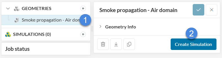
Hitting the ‘Create simulation’ button leads to the following options:
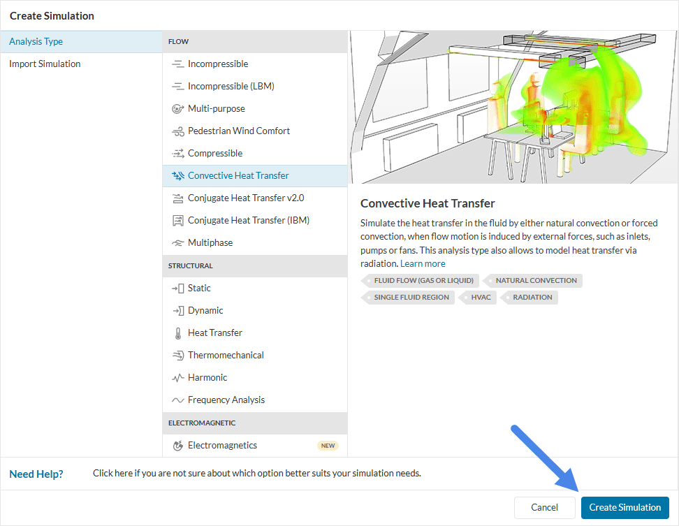
Choose ‘Convective heat transfer’ for analysis type and ‘Create the simulation’.
Now you can see the default simulation tree presented in the following picture:
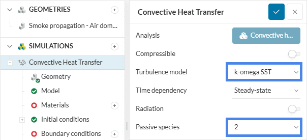
In the global simulation setup, please change the Turbulence model to ‘k-omega SST’. This model switches in between k-omega and k-epsilon automatically, therefore it takes advantage of both models.
Also, add 2 Passive species. These will help to define the sources of smoke from the chimneys and differentiate the concentration of them and clean air.
2. Set up the Simulation
In this part of the tutorial, we will define the physics of the model we want the solver to calculate.
2.1 Define a Material
This simulation will use ‘Air’ as fluid material. Therefore click on the ‘+ button’ next to Materials. In doing so, a library of fluid materials opens:
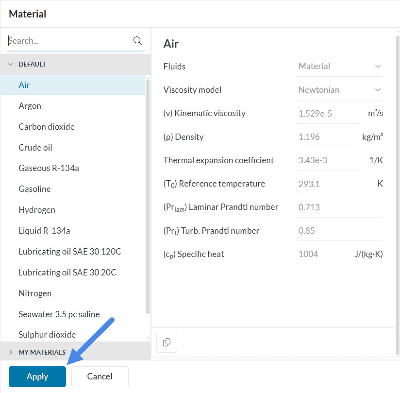
Select ‘Air’ and click ‘Apply’. In the window that opens, you can leave the default values and assign them to the entire flow region.
2.2 Model
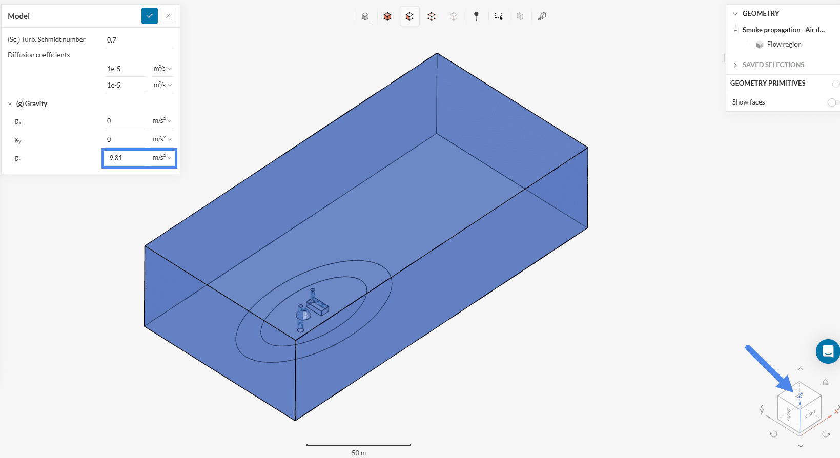
In the next step, we define gravity according to the global coordinate system. Therefore click on Model in the simulation tree.
For this geometry, the gravity direction is in the negative z-axis. Hence, input ‘-9.81’ in the z-direction. Leave the Diffusion coefficients and Turbulent Schmidt number as default.
gravity in G
2.2 Assign the Boundary Conditions
The following picture summarizes the boundary conditions applied in this simulation:
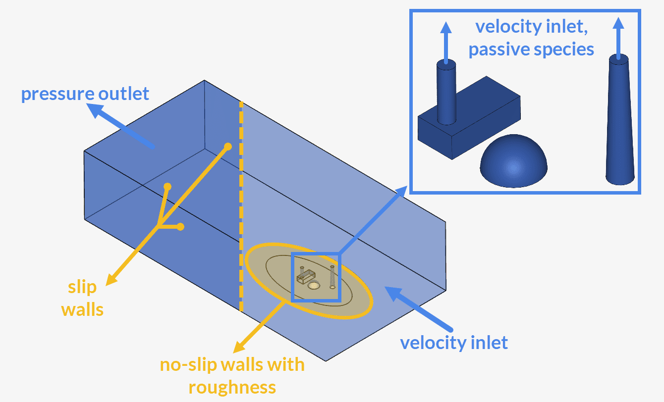
a. Walls – Slip
Follow the instructions presented in the picture below to add a new boundary condition:
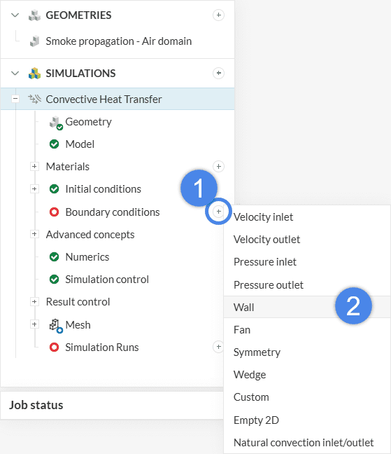
- After hitting the ‘+’ button next to boundary conditions, a drop-down menu will appear, where one can choose between different boundary conditions;
- Select the ‘Wall’ boundary condition.
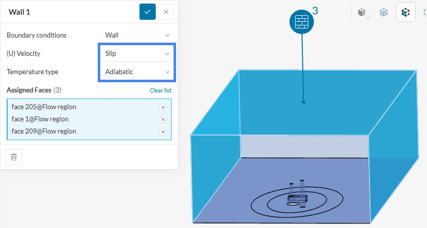
Change (U) velocity to ‘Slip’ and (T) Temperature to ‘Adiabatic’. Now assign the top, left, and right walls to this condition.
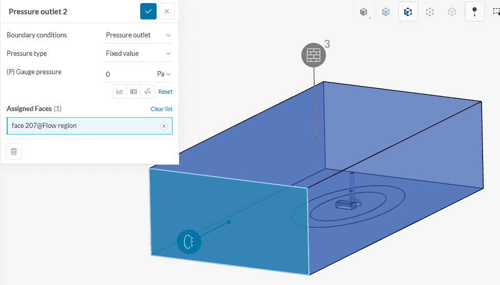
b. Pressure Outlet
Create a new boundary condition, but this time choose ‘Pressure outlet’. The outlet is further away from the chimneys.
c. Velocity Inlet – Chimneys
Create yet another boundary condition. Select ‘Velocity inlet’. Let’s first set up the inlet for the tall chimney.
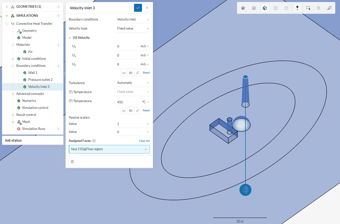
- Smoke will be released at ‘8 \(m/s\)’ in the z direction (Uz) and at
- A (T) Temperature of ‘450 \(°C\)’.
- The first passive species is therefore linked to the inlet flow from the tall chimney. That is why we select ‘1’ for the first Value within Passive scalars.
Set up another velocity inlet, this time for the short chimney:
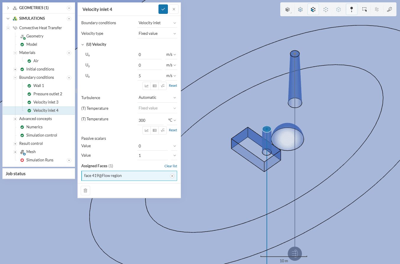
- Velocity will be ‘5 \(m/s\)’ in the positive z-direction.
- The temperature is ‘300 \(°C\)’.
- This inlet will receive a Value of ‘1’ for the second passive species.
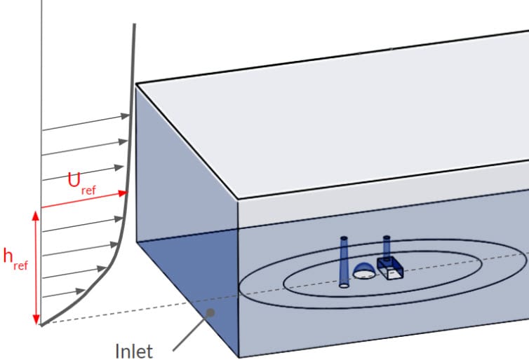
d. Velocity Inlet – ABL
In this step, we will set up an Atmospheric Boundary Layer (ABL). It consists of a pre-defined velocity profile, with a value zero on the ground, gradually increasing with height. In this tutorial, \(u_{ref}\) is 5 \(m/s\) and \(h_{ref}\) is 10 \(m\).
Refer to these equations for the formulation of the logarithmic profile:
This logarithmic profile has the following formulation:
$$u = \frac{u^{*}}{K} \cdot ln \left (\frac{z + z_{0}}{z_{0}} \right ) \tag{1}$$
Where
- ‘K‘ is the von Karman constant, equal to 0.41;
- ‘z0‘ is the aerodynamic roughness length. In this tutorial, we will consider it 0.03 meters;
- ‘z‘ is the height in which the velocity is calculated;
- ‘u*‘ is the friction velocity, given by:
$$u^{*} = K \cdot \frac{u_{ref}} {ln \left (\frac{z_{ref} + z_{0}} {z_{0}} \right )} \tag{2}$$
The turbulent kinetic energy (k) formulation is shown below. \(c_\mu\) is the turbulent viscosity constant, equal to 0.09:
$$k = \frac{{u^{*}}^{2}} {\sqrt{c_{\mu}}} \tag{3}$$
Finally, for the specific dissipation rate \(\omega\), the formula is:
$$\omega = \frac{u^{*}}{K \cdot \sqrt{c_{\mu}}} \cdot \frac{1}{z + z_{0}} \tag{4}$$
For more information about the setup parameters, please visit this page.
We will use formula inputs for \(u\), \(k\) and \(\omega\). Based on the equations above:
$$ u = \frac{5}{log \left (\frac{10 + 0.03}{0.03} \right) } log \left (\frac{z + 0.03}{0.03} \right) \tag{5} $$
$$ k = \left(\frac{0.41*5}{log \left (\frac{10 + 0.03}{0.03} \right)} \right)^2 \frac{1}{\sqrt{0.09}} \tag{6} $$
$$ \omega = \frac{5}{log \left (\frac{10 + 0.03}{0.03} \right)} \frac{1}{\sqrt{0.09}} \frac{1}{z + 0.03} \tag{7} $$
Follow the same procedure as presented in Figure 10 but choose a custom boundary condition:
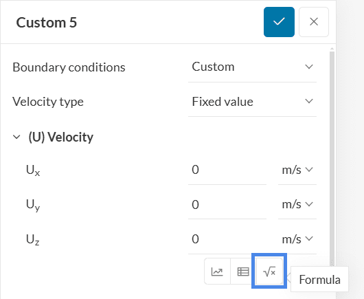
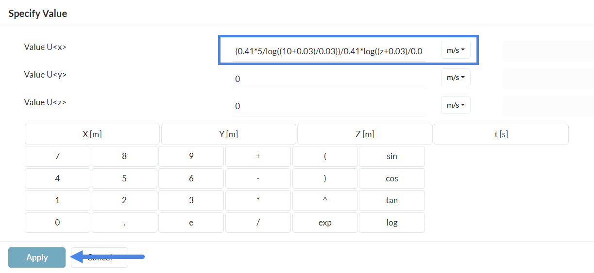
To input the formula for velocity, select a ‘Fixed value’, and then click on the highlighted button to open further options:
Afterward, two tabs will be available: Formula and Table. Switch to the formula input, and paste the velocity formula posted above in the x-direction. Hit ‘Apply’ to save.
Repeat the same process for \(k\) and \(\omega\). The other parameters should be as follows:
Formula for copy-paste
| Value | Formula |
| \((U)\) Velocity | (0.41*5/log((10+0.03)/0.03))/0.41*log((z+0.03)/0.03) |
| \((k)\) Turb. kinetic energy | ((0.41*5)/(log((10+0.03)/(0.03)))^2/(0.09)^0.5) |
| \( (\omega)\) Specific dissipation rate | (0.41*5/log((10+0.03)/0.03))/(0.41*(0.09)^0.5)*1/(z+0.03) |
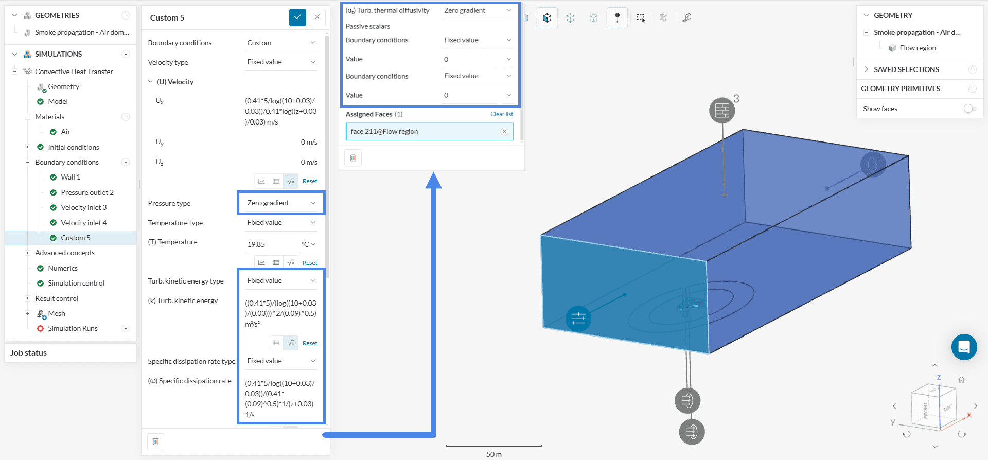
- Pressure type: ‘Zero gradient’;
- (T) temperature: ‘Fixed value’ at ‘19.85 \(°C\)‘;
- \(\alpha_t\) Turb. thermal diffusivity: ‘Zero gradient‘.
- Passive scalars: ‘Fixed value’ at ‘0’.
e. Building Walls
Solid walls will receive a no-slip condition. Furthermore, we can specify a surface roughness for the building walls, as well as for the terrains. For more information about the surface roughness model, check the relevant documentation.
Optional wall settings
The following custom boundary conditions, to define the surface roughness on building walls and the terrains, can be entirely skipped. This means that these surfaces will automatically receive a no-slip condition.
Create a Custom boundary condition.
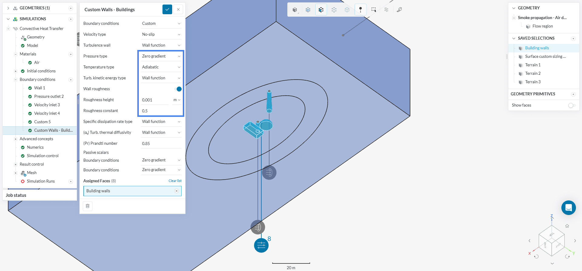
- Building walls will receive a Roughness height of ‘0.001 \(m\)’ with a
- Roughness constant of ‘0.5’.
- To save time, assign this boundary condition to a pre-created saved selection set named ‘Building walls‘:
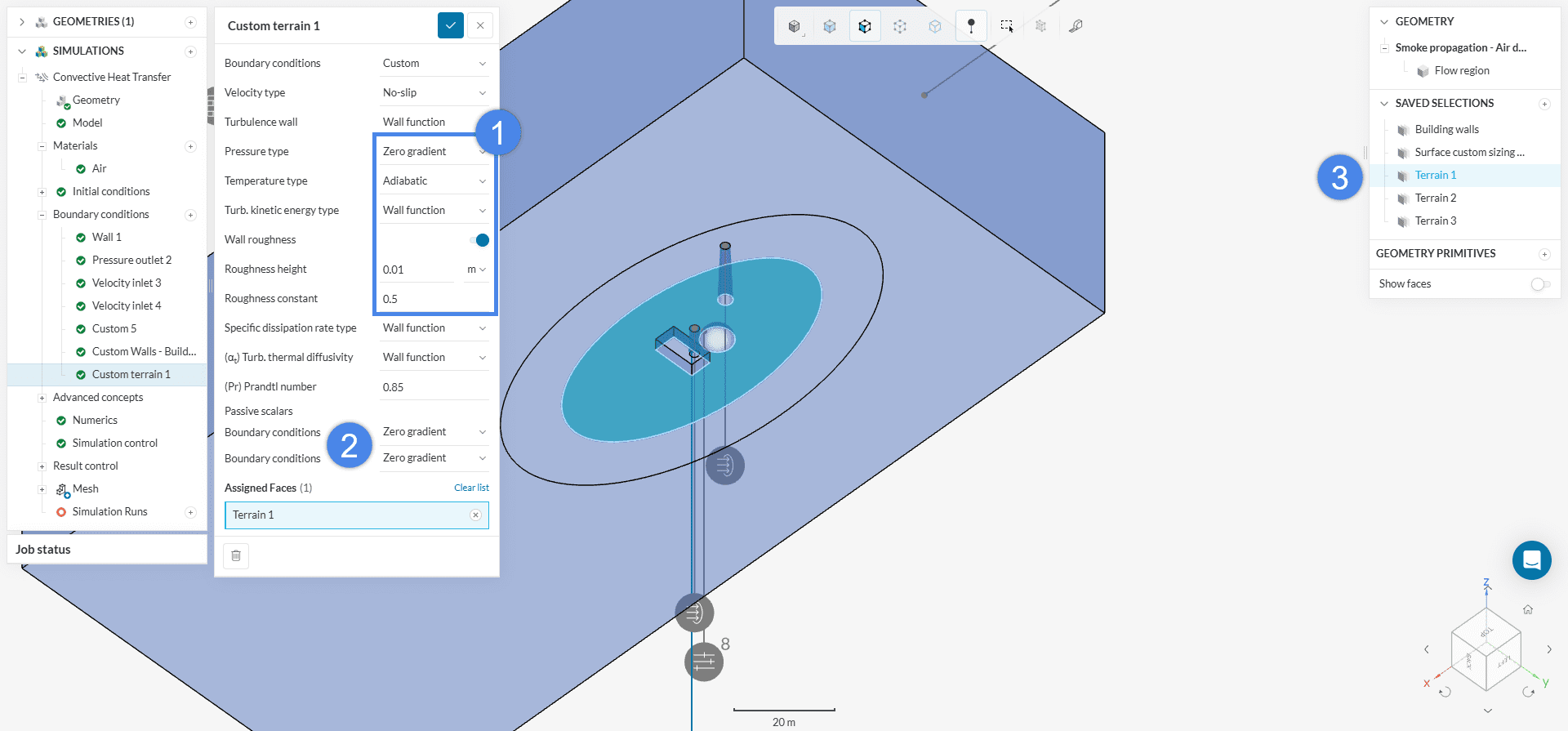
f. Terrains
The terrains will receive roughness as well. The custom boundary condition is the same as above. The only difference is the Roughness height:
- Terrain 1: Roughness height of 0.01 \(m\);
- Terrain 2: Roughness height of 0.0075 \(m\);
- Lastly, for terrain 3: Roughness height of 0.005 \(m\).
You can also use the pre-saved selection sets to correctly assign the terrains.
Repeat the same process for terrain 2 and 3.
Note
Check out this page, if you are interested in other boundary conditions available in SimScale.
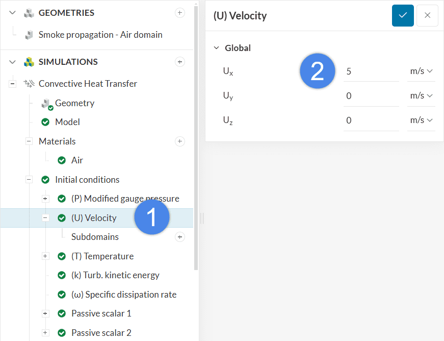
2.3 Initial Conditions
To enhance convergence, please initialize the velocity field with ‘5’ \(m/s\) in the x-direction. This velocity represents \(u_{ref}\):
2.4 Numerics and Simulation Control
The default settings for Numerics are optimized based on the analysis type. Therefore, they work well for most of the simulations and require no changes. However, if you are a simulation expert, you have full control over the settings and may change them as you like.
Access the Simulation control. Here we can define the number of iterations for the simulations as well as the write interval for specifying how many intermediate results to save.
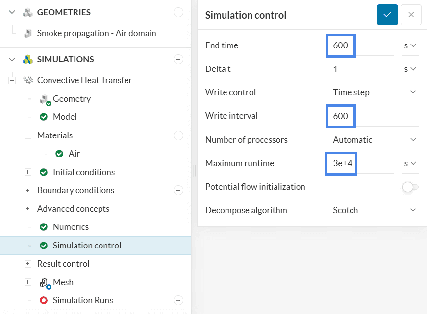
In Simulation control, change the End Time and the Write interval to ‘600’. Furthermore, please adjust the Maximum runtime to ‘30000’ seconds.
Note
For more information about simulation control and numerics, check the corresponding documentation pages.
2.5 Result Control
By setting result controls, you can observe the convergence behavior of several parameters of interest. Hence it is an important indicator to evaluate the quality and trustability of the results.
For this simulation, set up an Area average result control on the outlet. Please proceed as below:
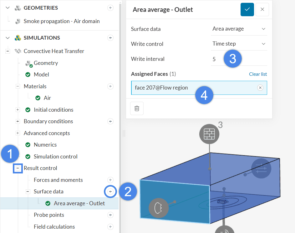
- Expand the Result control tab;
- Click on the ‘+ button‘ next to Surface data;
- Set Write interval to 5. This should be enough to see the convergence patterns;
- Assign it to the outlet face.
3. Mesh
To create the mesh, we recommend using the standard algorithm. This algorithm is a good choice in general, as it is quite automated and delivers good results for most of the geometries.
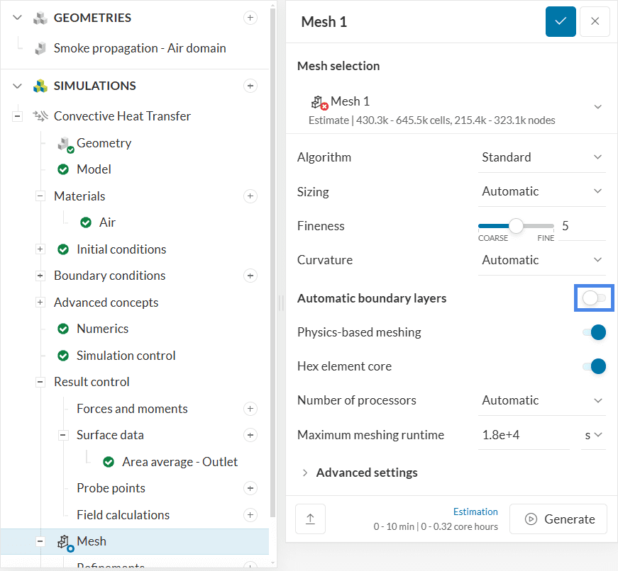
Disable Automatic boundary layers. The layers will be specified manually later. To improve the resolution around the areas of interest, we will set up three refinements.
3.1 Surface Custom Sizing Refinement
Click on the ‘+ button’ next to Refinements. The first refinement is Surface custom sizing. This refinement limits the maximum edge length of cells in chosen entities. Hence, it’s useful to improve the resolution in specific regions.
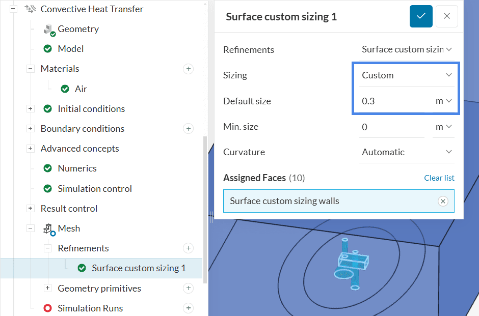
- Click on the ‘+ button’ next to Refinements.
- Set the Sizing to Custom
- Limit the Default size to 0.3 \(m\):
- To save time, assign it to a previously created saved selection set named Surface custom sizing walls. This set consists of the solid walls of the buildings and the smoke inlets. you can find it in the geometry panel on the right side of the Workbench.
3.2 Inflate Boundary Layer Refinement
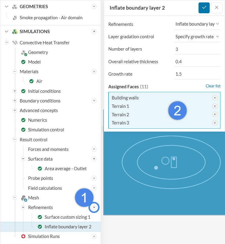
- Create an Inflate boundary layer refinement.
- Keep the settings as default and assign them to these 4 saved selection sets:
- Terrain 1, 2 and 3
- Building Walls
3.3 Volume Custom Sizing Refinement
To improve the resolution of the region around the chimneys, let’s create a Volume custom sizing refinement. Please proceed as below:
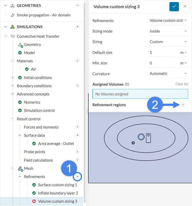
- First, create a Volume custom sizing refinement.
- Leave 1 meter as Default size and click on the ‘+ button’ to create a geometry primitive. Choose a Cartesian box and give it the following coordinates:
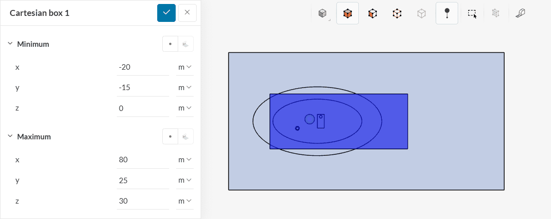
Finally, assign this cartesian box to the Volume custom sizing refinement. This step finalizes the setup of the simulation.
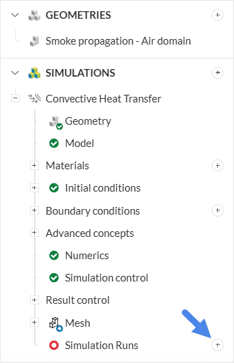
4. Start the Smoke Propagation Simulation
Click on the ‘+ button‘ next to Simulation runs and ‘Start‘ the process.
While it’s running, you can access the intermediate results by clicking on Solution fields. They’re updated as the iterations go by!
The entire smoke propagation simulation takes around 100 minutes to finish. In the reference project, which is linked below, we calculated a few more iterations, to assure complete convergence.
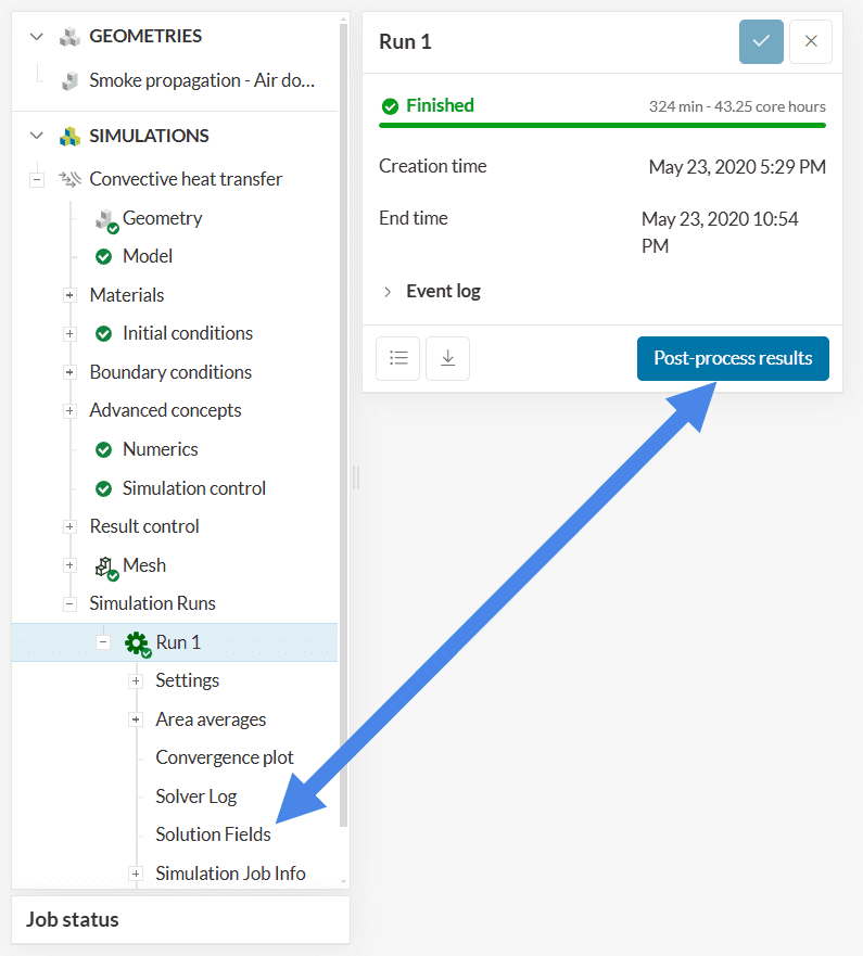
5. Post-Processing
5.1 Result Controls
Once the run is finished for your smoke propagation simulation, open the area average at the outlet result control. For steady-state simulations, the parameters are expected to converge and stabilize as iterations go on. Let’s inspect the average level of the first passive scalar (identified as T1):
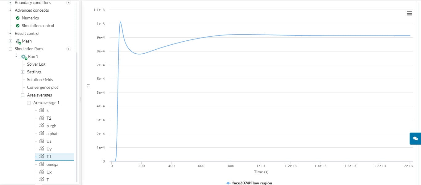
For this simulation, other parameters are also useful to assess convergence, such as velocity, temperature, and passive species levels at the outlet.
5.2 Particle Trace
The first post-processor filter that we will use is the ‘Particle Trace’ filter. This filter is very useful to know how the chimneys affect the airflow in the fluid domain. Please follow the steps below to visualize the particle traces:
- Toggle off the ‘Cutting Plane’ and create the Particle Traces by selecting the icon in th in the Filters panel and choose ‘Particle Trace’. This will take you to the settings of the particle trace.
- Next, place the seeds of the streamlines by clicking on the icon
 next to Pick Position. Place this at the inlet and align it with the height of the taller chimney. If you want to make sure the height of the seeds is appropriate, you can select the top and side enclosure walls, and hide them by right-clicking and choosing ‘Hide selection’.
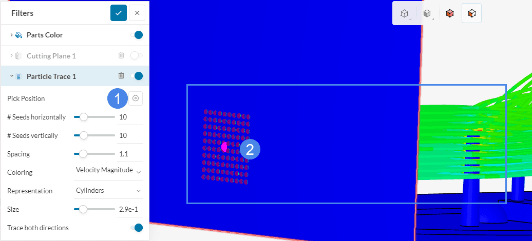
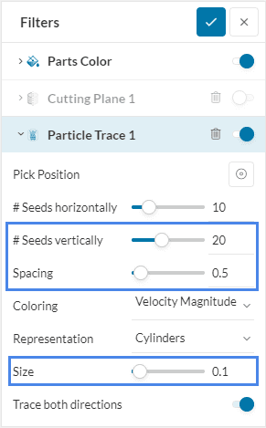
- Adjust the visualization of the streamlines. Increase the number of origin points by changing the #Seeds vertically to ’20’. Reduce the Spacing to ‘0.5’ and Size to ‘0.1’.
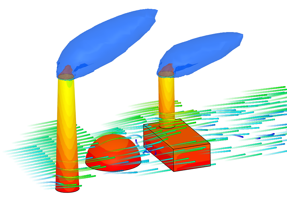
For the second chimney, you can repeat the same steps outlined above. As a result, the particle traces will be similar to the figure below:
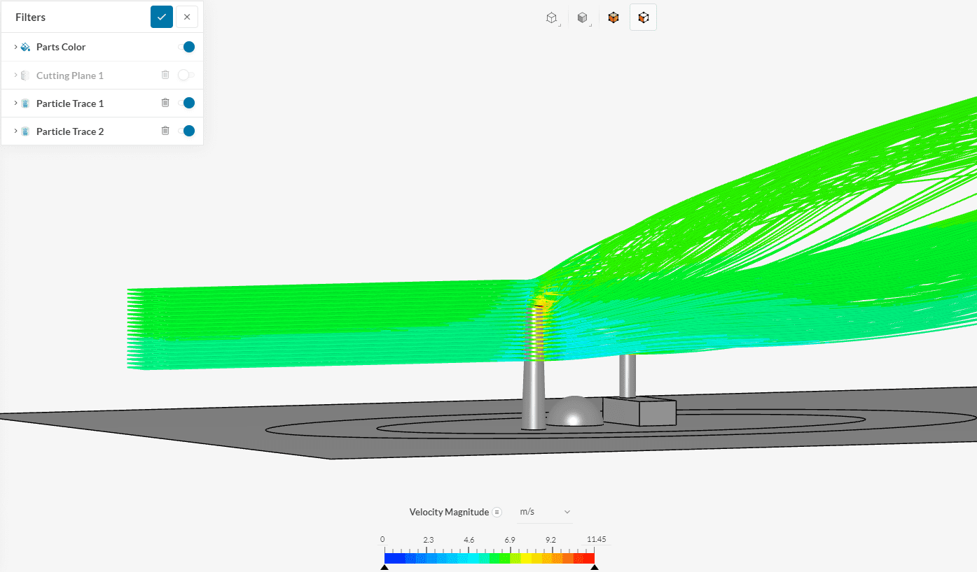
Based on Figure 35, the gas coming out of the chimneys causes the flow to rise and creates a higher velocity.
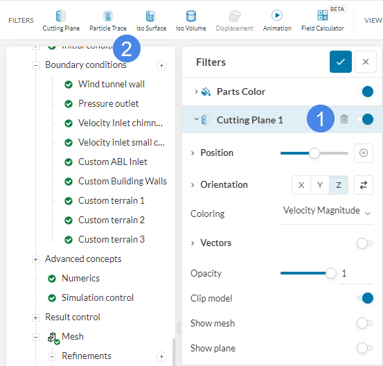
5.3 Cutting Plane
Next, let’s utilize a cutting plane generated by default to observe how the smoke propagation, or gas coming out of the chimneys, affects the temperature of the surroundings. Toggle the ‘Cutting Plane’ on and the ‘Particle Traces’ off. Set up the settings of the cutting plane by following the step below:
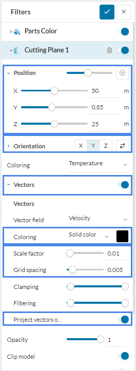
- Under Position, change the cutting plane placement by typing in the following coordinates: ’50, 0.85, 25′.
- The Orientation of the cutting plane should be in the ‘Y’ axis.
- Furthermore, please enable the velocity vectors with the on/off toggle next to Vectors.
- To improve the visualization, change the vectors’ Coloring to a black ‘Solid color’.
- Reduce the Scale factor to ‘0.01’ and the Spacing to ‘0.005’.
- To increase the visibility turn on the ‘Project vectors onto plane’.
After adjusting the setting the result should look similar to this:
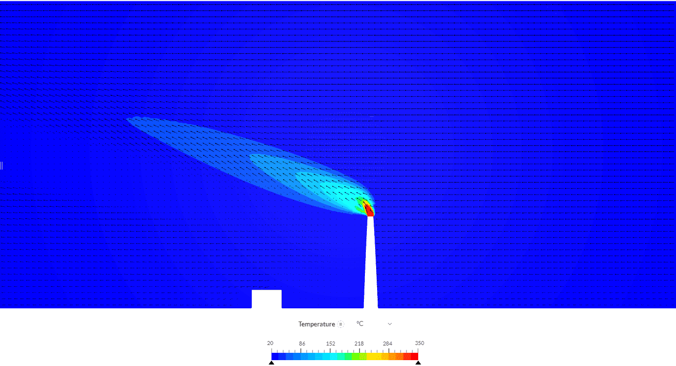
From the figure above, we can see that hot gas comes out of the chimney, affecting the air temperature downstream. The buoyancy effects are also noticeable, with the hot exhaust air quickly rising towards the top of the enclosure.
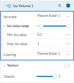
5.4 Iso Volume
The final filter that will be showcased is the Iso volume filter which is very useful to observe the propagation of the gases. Please follow the steps below to set an iso volume filter:
- Click the ‘Iso Volume’ button in the Filters panel.
- Change the Iso scalar and Coloring to ‘Passive scalar 1’ and the Min. iso value range to ‘0.1’ and the Max iso value to ‘1’. With these settings, we are going to highlight the volumes which consist of 10% to 100% of exhaust gases.
The settings for the Iso Volume 1 can be seen in the figure below:
- Follow the steps above for the gas coming out of the other chimney and changing the Iso scalar and Coloring to ‘Passive scalar 2’. The result should look similar to this:
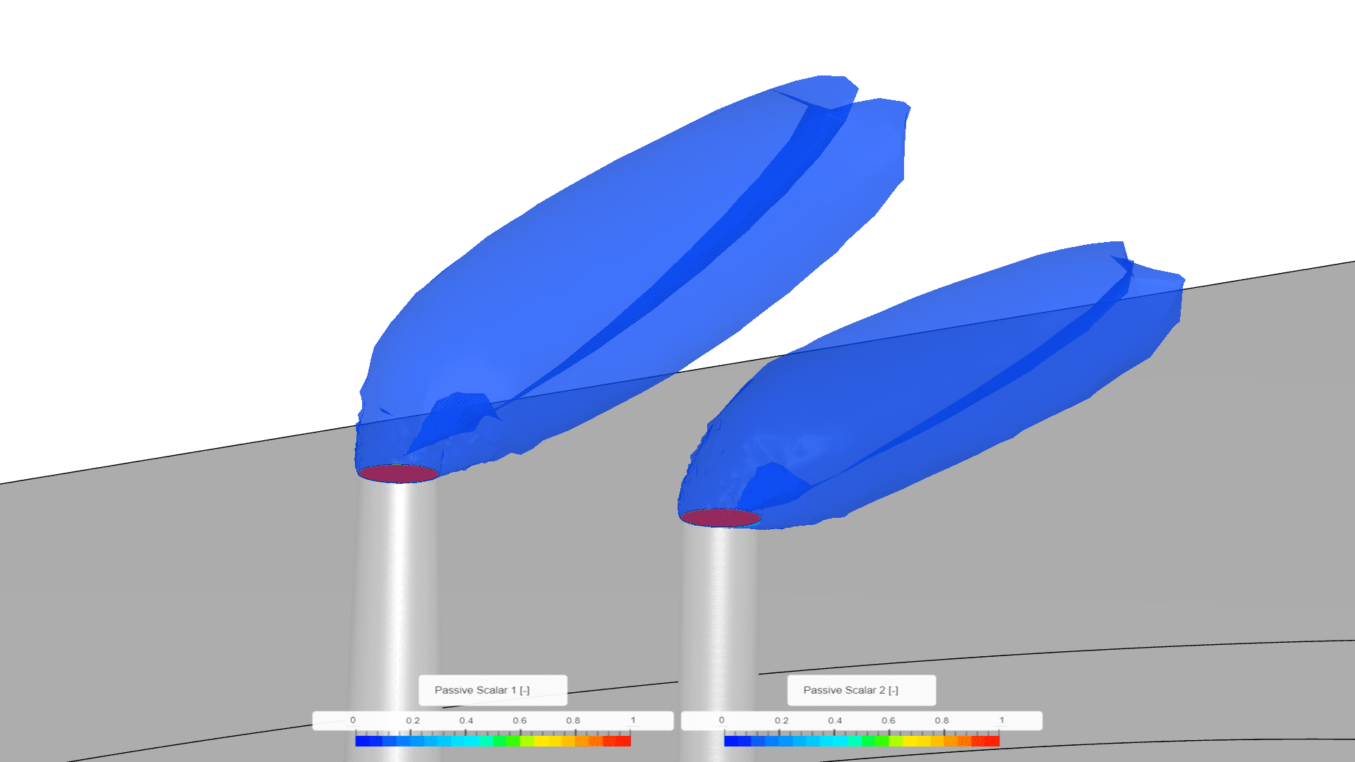
From Figure 39, you can see the smoke propagation results as the concentration of passive scalars. The Iso-Volume body displays the volume in which the smoke propagation is in a range from 0.1 to 1. It is evident that the smoke propagation is less than 10% as most of the higher concentration smoke remains at the boundary of the chimney outlet.
Analyze your smoke propagation results with the SimScale post-processor. Have a look at our post-processing guide to learn how to use the post-processor.
Congratulations! You finished the smoke propagation tutorial!
References
- Yang, Yi, et al. “Consistent Inflow Boundary Conditions for Modelling the Neutral Equilibrium Atmospheric Boundary Layer for the SST k-ω Model.” Wind and Structures, vol. 24, no. 5, 2017, pp. 465–480., DOI:10.12989/was.2017.24.5.465.
Note
If you have questions or suggestions, please reach out either via the forum or contact us directly.
Last updated: April 6th, 2026
Did this article solve your issue?
How can we do better?
We appreciate and value your feedback.


