How do I Model a Fan Curve in SimScale?

This Knowledge Base article describes the steps to implement a fan curve in SimScale.

A fan is a mechanical machine used to generate fluid flow. As the flow rate increases, the pressure drop in the system also increases, which affects the performance of the fan. Fan manufacturers provide a fan curve that describes the relationship between static pressure, power demand, speed, and efficiency values per-flow rate. This information is very important for cooling purposes, which is why we need to model the fan curve when possible.

Approach

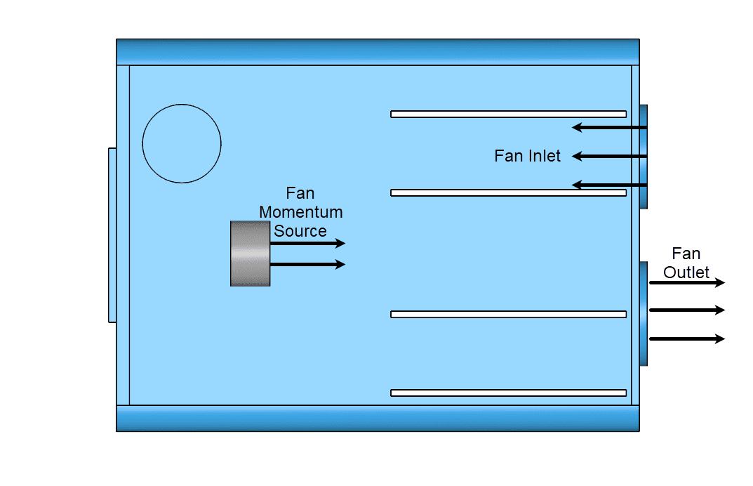
On the SimScale platform, two methods are used to implement a fan curve in the simulation. To simulate an external fan, which is located outside the fluid region, the fan curve can be assigned as a boundary condition. This can be done either as an inlet for an intake fan or as an outlet for an extraction fan. If the fan is located within the fluid region and therefore no boundary condition can be used, a momentum source can be assigned to a representative volume to induce the pressure jump created by the fan onto the flow field.

1. Analysis Types

The fan boundary condition and fan momentum sources advanced concept can be assigned to these analysis types:

• Incompressible
• Compressible
• Convective Heat Transfer
• Conjugate Heat Transfer v2.0
• Immersed Boundary

2. External Fan Boundary Condition

When a fan is attached to the fluid region the fan curve can be defined as a boundary condition. This can either push air into the fluid domain or create suction to extract air from the fluid region. To create a fan boundary condition please follow the steps below.

1. Create a ‘Fan’ boundary condition by hitting the ‘+’ button next to Boundary conditions.
2. Define the values according to the following figure:

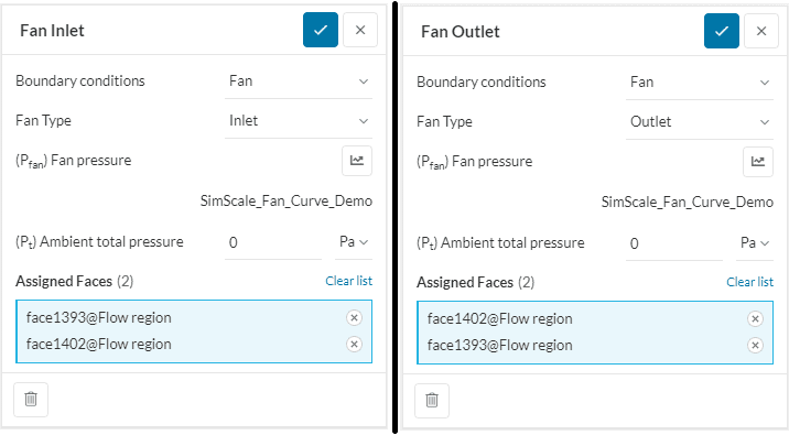
• Fan Type: ‘Inlet‘ or ‘Outlet’. Assign the flow direction of the fan. Use ‘Inlet’ for flow into the fluid domain and ‘Outlet’ for flow out of the fluid domain.
• \( (P_{Fan}) \) Fan pressure: Setup the fan curve or upload a .csv file. Note that the fan pressure is based on total pressure values.
• \( (P_{t}) \) Ambient total pressure: Assign the ambient pressure of the environment.
• Temperature type: ‘Inlet’. When defined in a heat transfer analysis the inlet temperature has to be set for the inlet flow.
• Assigned Faces: Assign all faces to which the boundary condition should be applied to. Each face will be treated as an individual fan.

3. Internal Fan Momentum Source

When a fan is inside the fluid domain a fan momentum source can be used to induce the pressure jump created by the fan onto the flow field. For this, a separate geometry has to be created to assign the mesh to the representative fan volume. The volume used for this assignment can either be a geometry primitive or directly generated in the CAD mode. To create a fan momentum source please follow the steps below:

1. Create a ‘Fan Model’ boundary condition by hitting the ‘+’ button next to Momentum Sources under Advanced Concepts.
2. Define the values according to Figure 4:

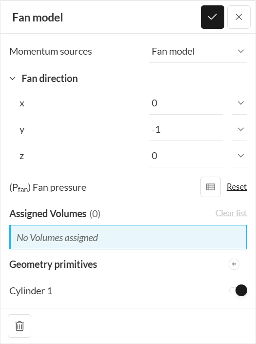
• Fan Direction: Create the vector to specify the direction of the fan.
• \( (P_{Fan}) \) Fan pressure: Setup the fan curve or upload a file. Note that the fan pressure is based on total pressure values.
• Assigned Volumes: Assign the volume which represents the fan geometry.

4. Fan Curve

On the SimScale platform, a fan curve can either be created by filling in the table with the volumetric flow rate and pressure, or by uploading a .csv file, containing this information.

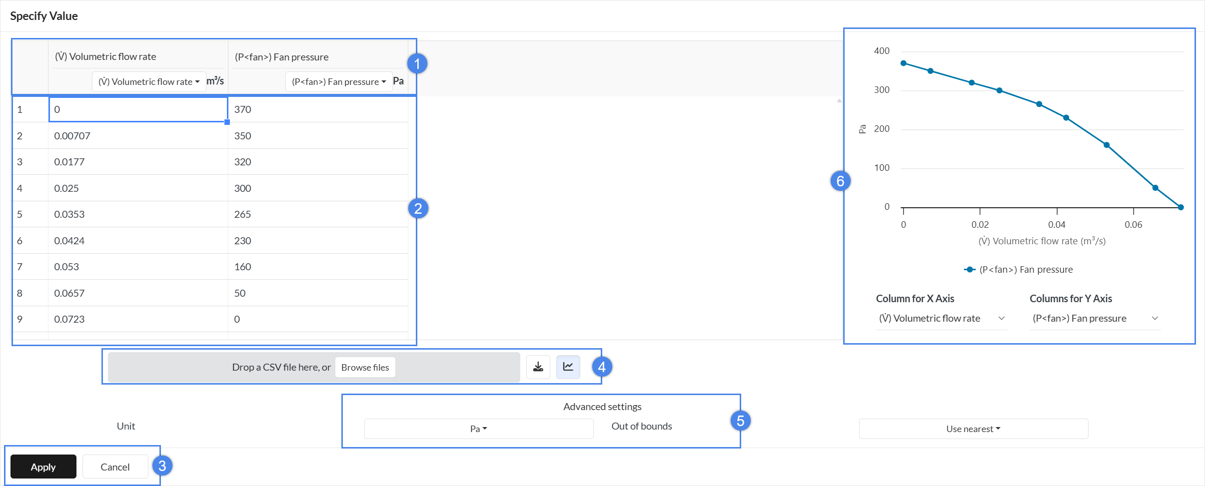
1. Set the assignment of the volumetric flow rate and the fan pressure to the corresponding line of your data set.
2. Enter custom values to the fan curve list.
3. Save the fan curve by selecting ‘Apply’ or abort any changes by selecting ‘Cancel’.
4. Upload a .csv or drag and drop a .csv into the dark grey area. You can also download the generated table as a .csv file, by clicking the download icon next to the Browse Files section.
5. Expand the Advanced settings to change the unit format for the fan pressure.

Figure 6 shows an example of the structure of a .csv file:

Make sure to have two columns: One representing the volumetric flow rate, and the other one the fan pressure. Assign the flow rate and pressure headers as well as the correct units to the corresponding columns. In the picture above, column A is the flow rate and column B is the fan pressure.

Expected Outcome

The following figures show the different effects of the fan pressure applied to an electronic box for the different methods of implementing a fan curve in SimScale.

Figure 7 shows the flow direction and velocity distribution on a plane cut through the fluid domain for the fan inlet situation:

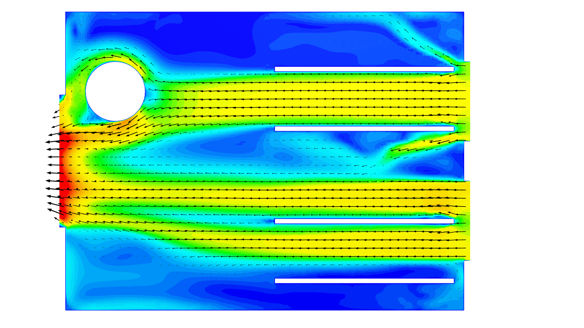
Figure 8 shows the flow direction and velocity distribution on a plane cut through the fluid domain for the fan outlet situation:

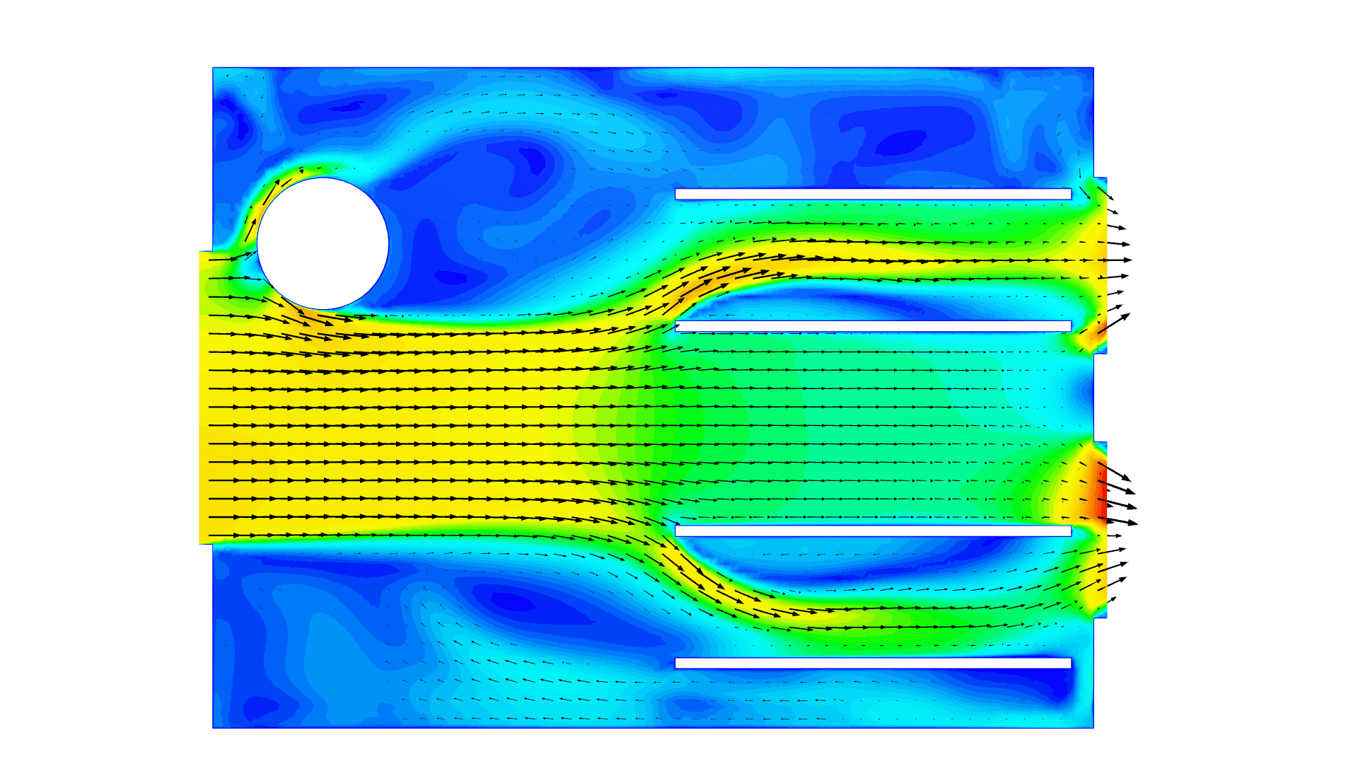
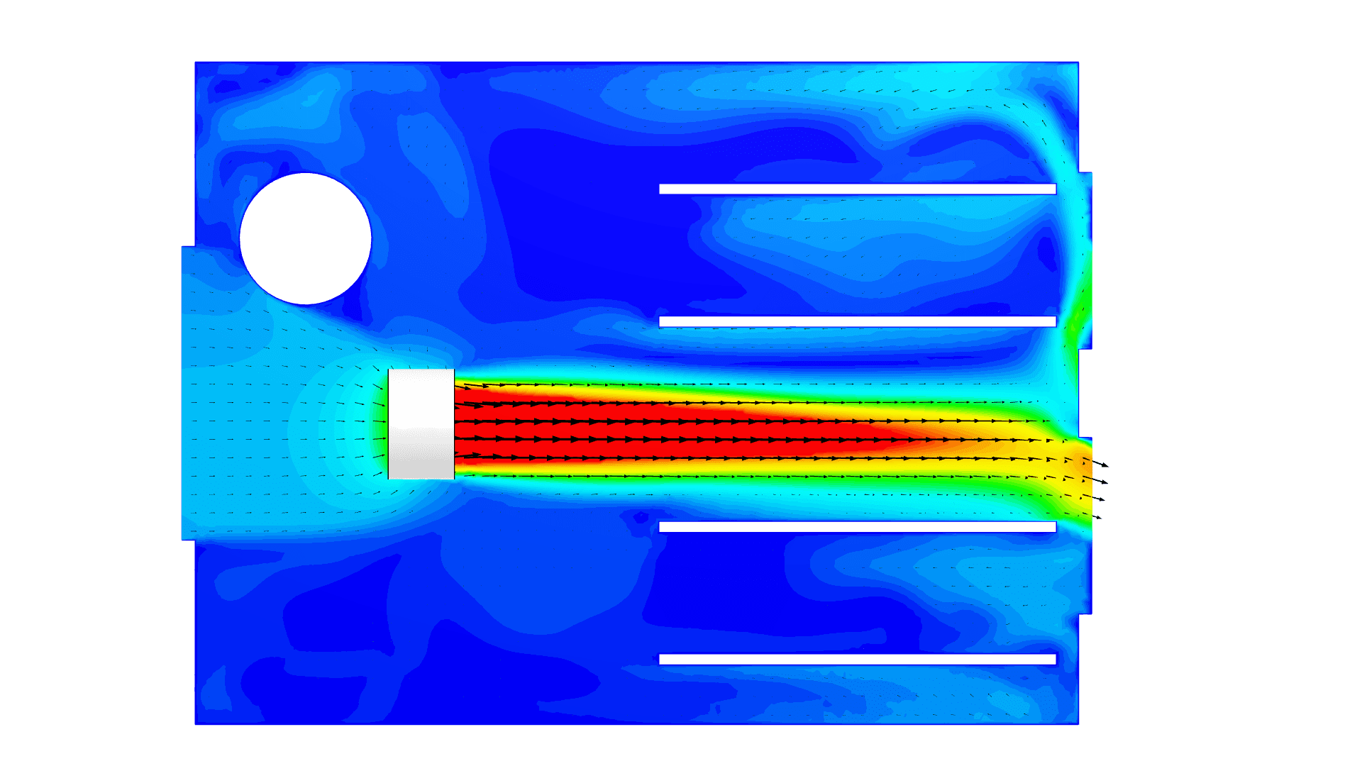
Figure 9 shows the flow direction and velocity distribution on a plane cut through the fluid domain for the fan momentum source condition situation:

5. Reference Project

A reference project showing all different implementations is linked below:

Custom Boundary Condition Method

In addition to the predefined boundary conditions, SimScale also offers the option to create a custom boundary condition which brings more options to implement a fan curve. To create a custom boundary condition please follow the steps below.

1. Create a custom boundary condition by hitting the ‘+’ button next to Boundary conditions (BC).
2. Select ‘Custom’.
3. Define the values according to the following figure:

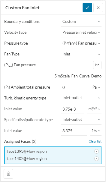
• Velocity type: ‘Pressure inlet-outlet velocity‘. This means that the velocity on the fan BC is dependent on the pressure difference. If the pressure difference between the inlet and the outlet is negative, the flow will leave the system (the reverse direction).
• Pressure Type: ‘(P<fan>) Fan pressure’. Using this setting, the user can upload a fan curve.
• Fan type: ‘Inlet’ is an intake fan, therefore flow should come into the system. ‘Outlet’ is an exhaust fan, therefore flow should come out of the system
• \( (P_{Fan}) \) Fan pressure: Upload a fan curve or create a new fan curve.
• \( (P_{t}) \) Ambient total pressure: If the ‘Compressible‘ toggle is on, assign the absolute pressure. Else, assign the gauge pressure.
• Turb. kinetic energy type: ‘Inlet-outlet’. If the fluid leaves the system, the turbulent kinetic energy value at the inlet will be calculated by the solver. If the fluid enters the system, the user-defined Inlet value will be considered instead.
• Specific dissipation rate type: ‘Inlet-outlet’. If the fluid leaves the system, the specific dissipation rate value at the inlet will be calculated by the solver. If the fluid enters the system, the user-defined Inlet value will be considered instead.
• Temperature type: ‘Inlet-outlet’. If the fluid leaves the system, the temperature value at the inlet will be calculated by the solver. If the fluid enters the system, the user-defined Inlet value will be considered instead.