Tutorial: Drone Simulation Using Rotating Zones

This article provides a step-by-step tutorial for the flow simulation around a drone using rotating zones (the propeller) using the moving reference frame (MRF) modelling technique.

flow visualization drone simulation mrf rotating zone — Figure 1: Flow visualization across the drone rotating propeller

This tutorial teaches how to:

Set up and run an incompressible flow simulation
Assign boundary conditions, material, and other models to the simulation
Mesh the geometry with the SimScale standard meshing algorithm
Set up a moving reference frame (MRF) rotating zone

The typical SimScale workflow will be followed:

Prepare the CAD model for the simulation
Set up the simulation
Set up the mesh
Run the simulation and analyze the results

1. Prepare the CAD model and Select the Analysis Type

First of all, click the button below. It will copy the tutorial project containing the geometry into your Workbench.

Import Tutorial into Workbench

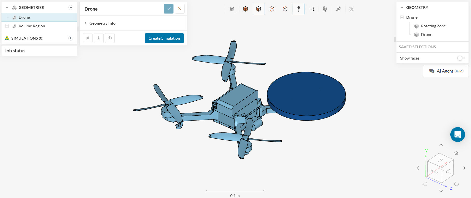
The following picture demonstrates what should be visible after importing the tutorial project:

imported project drone simulation mrf rotating zone — Figure 2: View of the imported project in the SimScale Workbench

1.1 Required CAD Preparation: Rotating Zones

You can see that there are two geometries in the imported project. The first one is called Drone and the second one is called Volume Region. The drone model shows the body with its four propellers and a cylinder surrounding the region that will rotate:

drone geometry including the rotating zone cylinder simscale — Figure 3: The original drone body with its four impellers. Due to symmetry, only one impeller will be simulated.

An important optimization in the simulation is achieved by noticing that this model has two planes of symmetry. This means that we can get away with modelling only one-quarter of the geometry. This is performed in the creation of the bounding box, which covers the desired quarter as shown in the following picture:

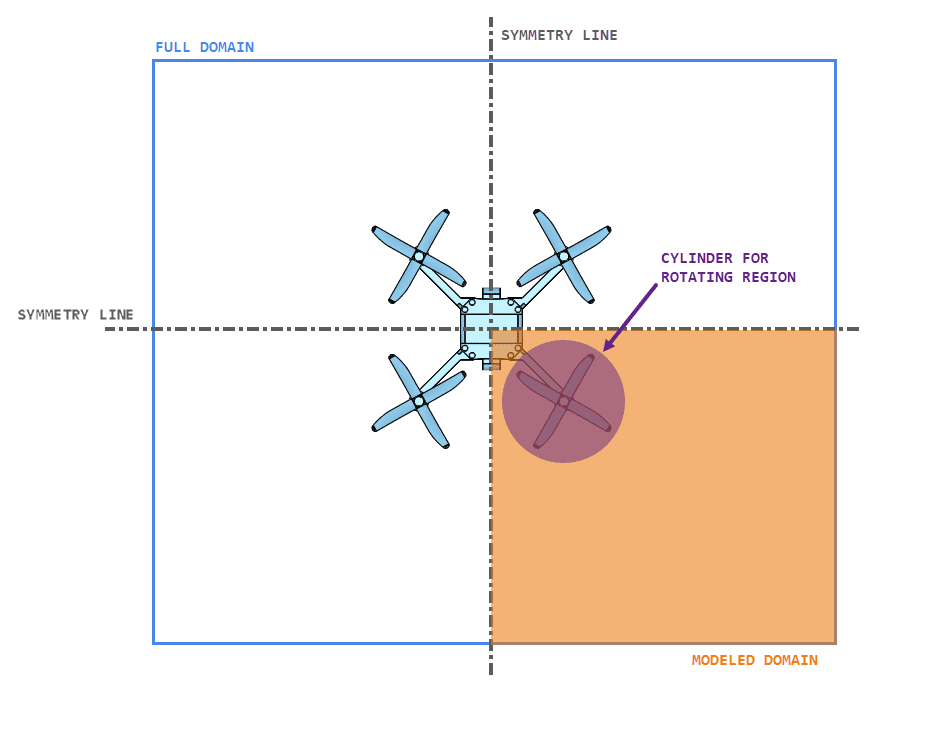
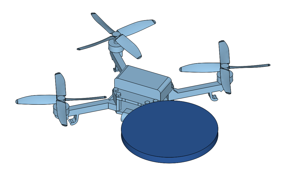
symmetry model drone simulation mrf rotating zone — Figure 4: Modeled domain, symmetry, and cylinder for rotating region.

A crucial aspect of the modelling is the creation of the cylinder for the rotating region. This cylinder should cover (with some margin) the faces that will be included in the rotation model. The one used in our case covers the drone propeller, and can be found by having a closer look at the Drone Parts geometry:

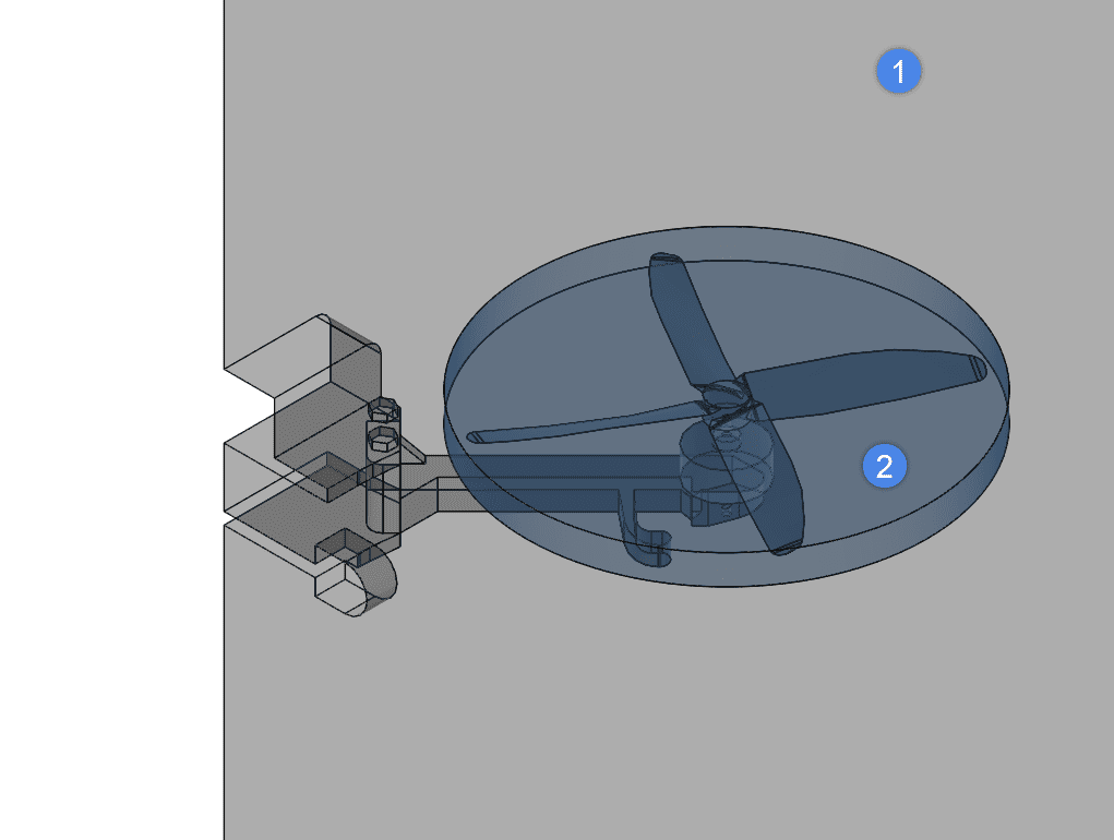
geometry detail drone simulation mrf rotating zone — Figure 5: Detail of the geometrical volumes present in the model

The flow region (gray), which models the volume filled by fluid. Notice that it has a void representing the space occupied by the drone structure and propellers and that it uses the symmetry of the model as explained above.
A cylinder covering the propeller (blue). This cylinder will be used to create the region of cells rotating and the MRF concept.

Tip

You can better visualize the internal faces by changing the render mode to translucent surfaces. Do this by using the top bar at the viewer.

Important

In case you want to model your drone or any external rotating geometry for that matter, you should always follow the modelling convention outlined in this section: a flow region volume with the removed bodies and a cylinder around the rotating region.

You can also create the flow region using CAD mode, or in your CAD following the instructions on this page.

1.2 Create Saved Selections

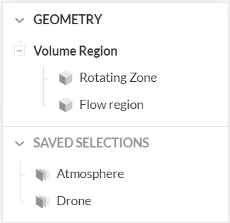
Saved Selections are groups of faces used for quickly applying boundary conditions or other assignments. Such selections are listed in the panel on the right side of the Workbench.

For example, the Volume Region geometry has a couple of pre-saved selections:

saved selections for drone simulation with mrf rotating zone — Figure 6: Set of saved selections

For the Volume Region geometry, please create a new saved selection for the symmetry planes, following the steps below:

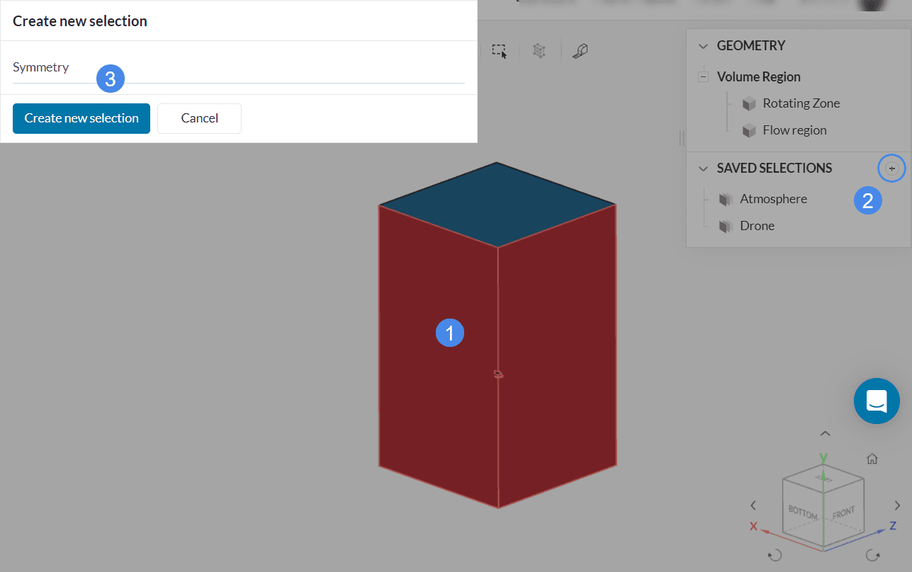
creating saved selections for drone simulation with mrf rotating zone — Figure 7: Creating saved selections

First, select the corresponding two faces from the viewer (notice these are the ones that intersect with the drone).
Click the ‘+’ icon next to Saved Selections in the right-hand side panel.
In the pop-up dialog that appears, name the selection ‘Symmetry’ and click on ‘Create new selection’.

1.3 Create the Rotating Zones Drone Simulation

Now we can start with the simulation setup. Follow the steps presented in the picture below to create a new simulation for our geometry:

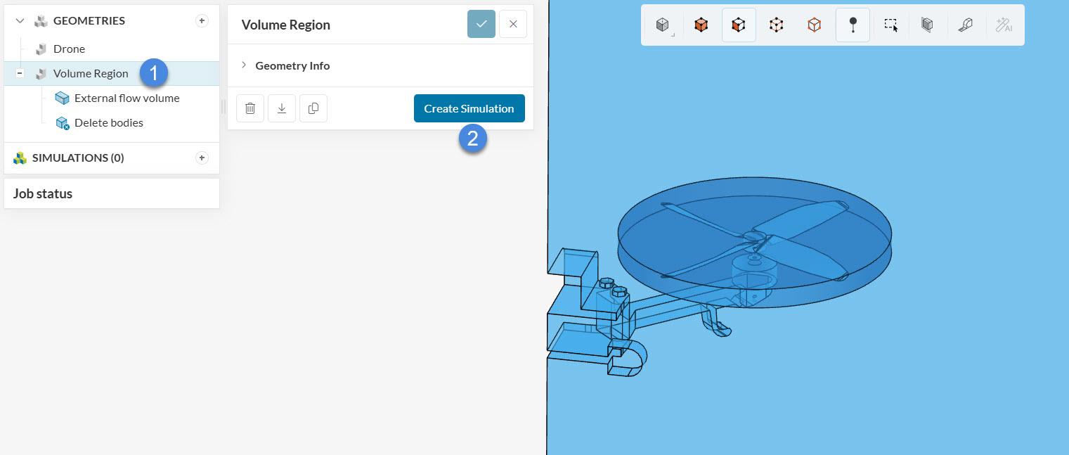
create simulation drone simulation mrf rotating zone — Figure 8: Creating a new simulation

Select the ‘Volume Region’ geometry from the left panel
Click on the ‘Create Simulation’ button

At this point, the analysis type selection widget appears:

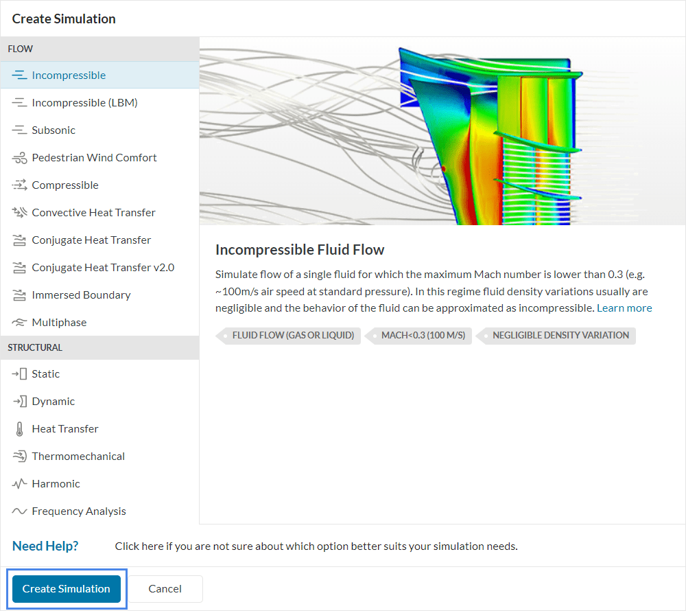
simulation library drone simulation mrf rotating zone — Figure 9: SimScale simulation library

Choose ‘Incompressible’ and click on ‘Create Simulation’. A new simulation tree will appear at the left panel and a pop-up with the global simulation settings, which we will leave at the default values.

2. Set Up the Rotating Zones Simulation

2.1 Material Model

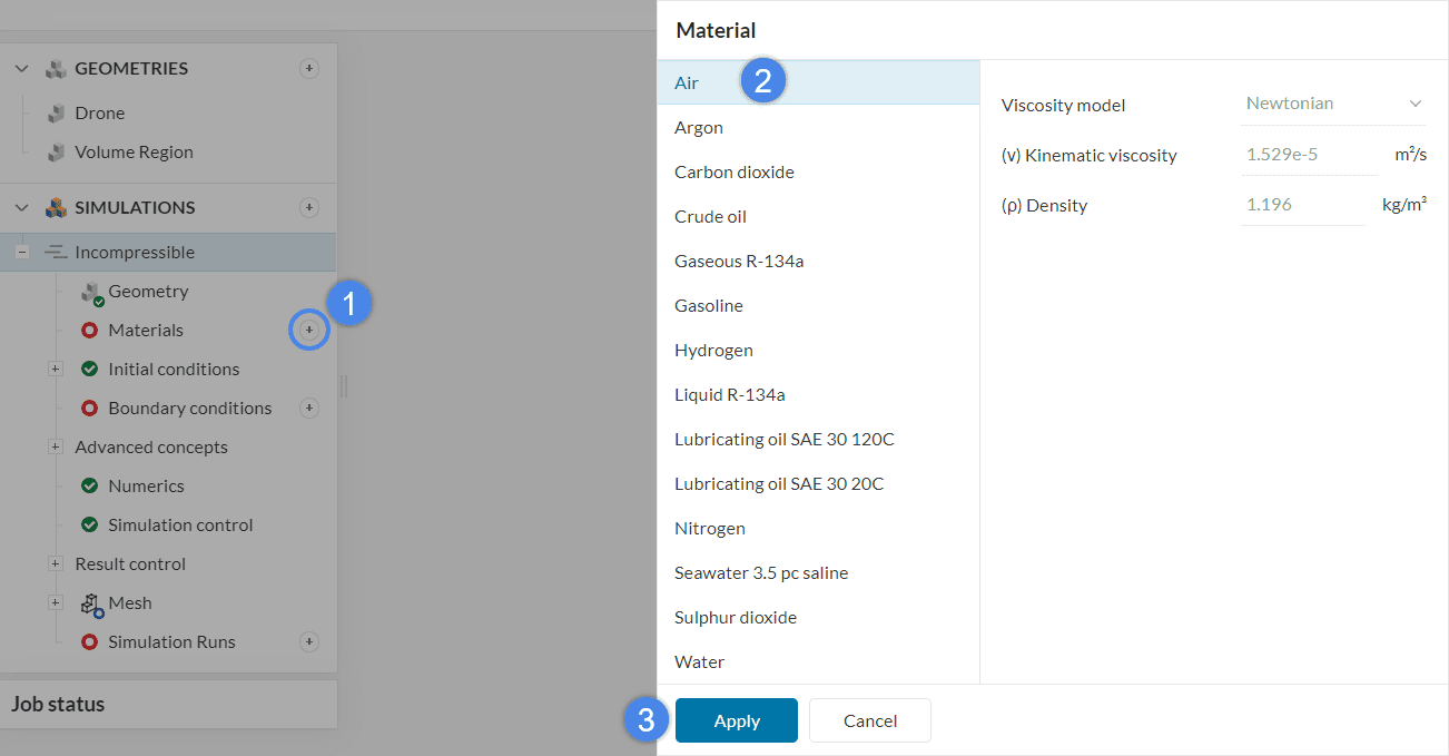
To define and assign a material, click the ‘+’ button next to Materials. Doing so, the SimScale material library will pop up. Select Air from the materials library and click Apply:

materials library drone simulation mrf rotating zone — Figure 10: SimScale materials library

The material properties window will appear. Assign the Flow Region volume and accept the selection with the check-mark button.

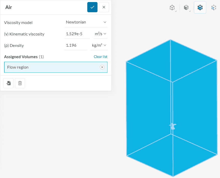
materials properties drone simulation mrf rotating zone — Figure 11: Material parameters for air and assignment of the flow region

Please note that only the flow region receives a material definition -the Rotating Zone volume remains without an assignment.

2.2 Boundary Conditions

Now we will define the boundary conditions. To create a boundary condition, follow the steps shown in the picture below:

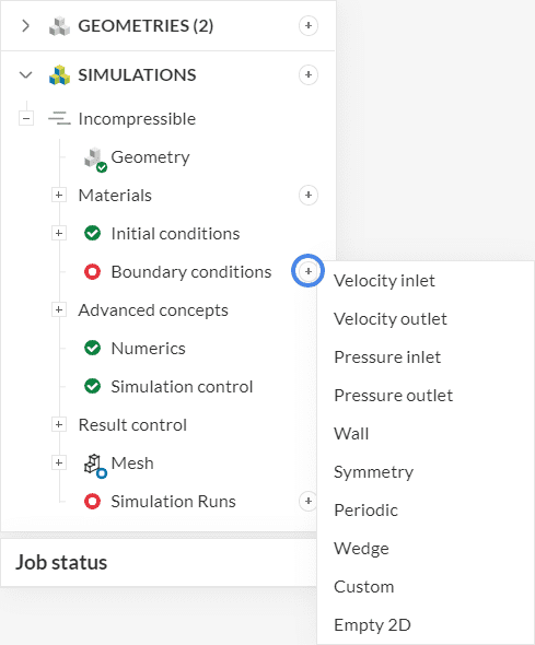
creating boundary condition drone simulation mrf rotating zone — Figure 12: Creating a boundary condition

Click on the ‘+’ button next to Boundary Conditions
Select the proper type from the drop-down menu
Set up the physical parameters and assigned faces in the pop-up dialog (not shown in the picture)

Now apply this process for the following boundary conditions:

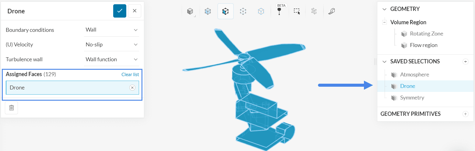
a. Drone Surface

For the drone faces, a no-slip wall condition is used.

Create a new boundary condition by following the instructions in Figure 12 and selecting ‘Wall’. Now select the Drone saved selection to assign it to the boundary condition. You can also rename the boundary condition to ‘Drone’.

Leave all parameters as default, as shown in the picture:

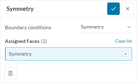
drone faces boundary condition drone simulation mrf rotating zone — Figure 13: Wall boundary condition for the drone faces

b. Symmetry Planes

For the symmetry planes, a ‘Symmetry’ boundary condition is used.

Create it according to the steps presented in Figure 12. Once the setup panel pops up, select the Symmetry saved selection that was created before for the assignment.

The setup should look as shown in the picture:

symmetry planes boundary condition drone simulation mrf rotating zone — Figure 14: Symmetry plane boundary condition

c. Atmosphere

For the faces open to the atmosphere, a custom boundary condition will be used. Follow the same procedure as before to create a custom boundary condition.

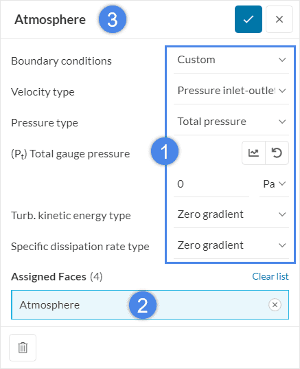
creating a custom atmospheric boundary condition in simscale — Figure 15: Custom inlet-outlet boundary condition for the faces open to atmosphere

As we do not know if the direction of flow at these faces will be inlet or outlet, it will allow the solver to automatically compute it. Therefore we select ‘Pressure inlet-outlet velocity’ for the (U) Velocity setup.
- Define ‘Total pressure’ for the gauge pressure option and assign ‘0’ Pa, which corresponds to atmospheric pressure.
- We set the turbulence quantities, Turb. kinetic energy and Specific dissipation rate to ‘Zero gradient’, so that the solver calculates them.
Now assign the ‘Atmosphere’ saved selection to the boundary condition.
If you want you can also rename the boundary condition to ‘Atmosphere’ to keep the setup more organized.

2.3 Propeller Rotation

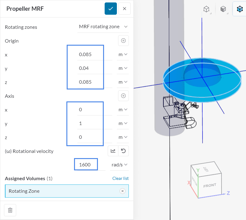
To specify the rotating propeller in our model, a moving reference frame (MRF) rotating zone is employed. The following picture shows how to create it:

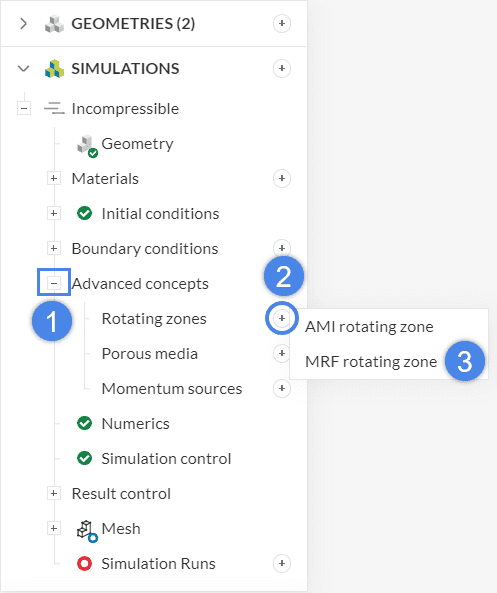
creating rotating zone drone simulation mrf rotating zone — Figure 16: Creating an MRF rotating zone

Expand Advanced concepts.
Click on the ‘+’ button next to Rotating zones.
Select ‘MRF rotating zone’ from the list.

In the pop-up window, assign the Rotating Zone volume and set up the parameters as shown in the picture:

setup of mrf rotating zone — Figure 17: Creating the MRF rotating zone.

You can read more on the topic of MRF rotating zones at the corresponding documentation page:

Rotating Zones

2.4 Numerics and Simulation Control

For the numeric solver parameters, one parameter will be changed: The Number of non-orthogonal correctors. This will allow the solver to achieve a better solution for the tetrahedral mesh created by the SimScale standard mesher algorithm:

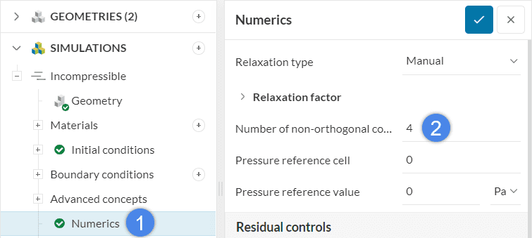
numerics parameters drone simulation mrf rotating zone — Figure 18: Numerics setup. Set the *Number of non-orthogonal correctors* to ‘4’.

Select Numerics from the tree at the left panel.
Set the Number of non-orthogonal correctors to ‘4’.

The Simulation control parameters are left as default.

3. Mesh

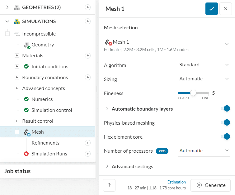
For the mesh setup, all settings are left as default, as we will make use of the SimScale standard mesh algorithm. You do not need to click Generate either, as the mesh will be computed as part of the simulation run:

mesh parameters drone simulation mrf rotating zone — Figure 19: Mesh setup

Did you know?

It’s necessary to define cell zones in the mesh whenever we want to apply a specific property, such as a rotating motion, to a subset of cells.

The standard mesher algorithm automatically creates the necessary cell zones whenever Physics-based meshing is enabled. Since we are using physics-based meshing in this tutorial, the algorithm will take care of the cell zone definition.

If you are using a different mesher, you can learn alternative ways to define a cell zone on the rotating zones documentation page.

4. Start the Rotating Zones Simulation

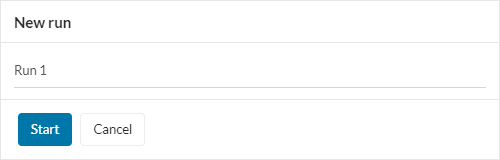
Now that the simulation setup is complete, a new simulation run can be created to perform the computation. To do so, click the ‘+’ button next to Simulation Runs at the left panel. In the pop-up window, give a proper name to the run and click ‘Start’:

creating simulation run drone simulation mrf rotating zone — Figure 20: Creating and starting a new simulation run

This computation takes around 30-40 minutes to be completed. If you can’t wait to see the results, at the end of the article you will find a link to the completed version of the project.

5. Post-Processing

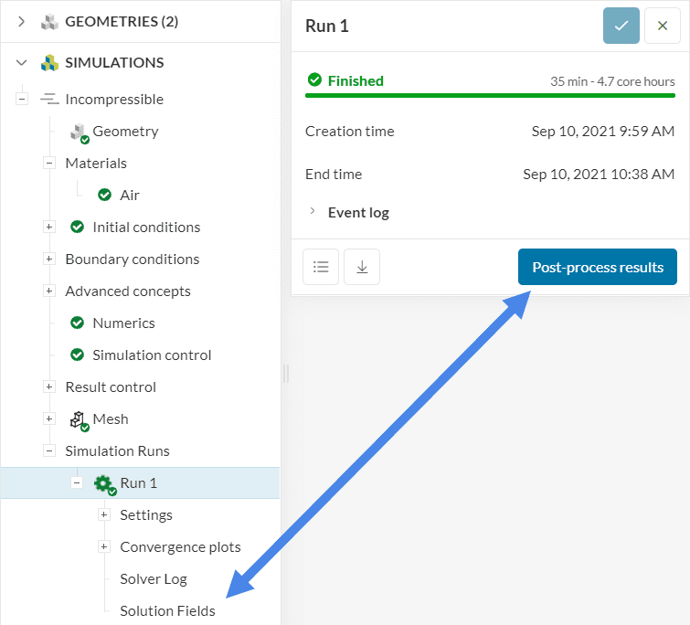
After the simulation is finished, access the post-processor by clicking the ‘Post-process results’ button or ‘Solution Fields’ under your run.

access to the post-processor — Figure 21: Click **‘Post-process results’** in your *Run* dialog or **‘Solution Fields’** under your run to access the post-processor.

5.1 Surface Visualization

One of the most important things to observe in the drone is the pressure distribution on the surfaces of the drone. Follow the steps below to show pressure on the surfaces of the drone:

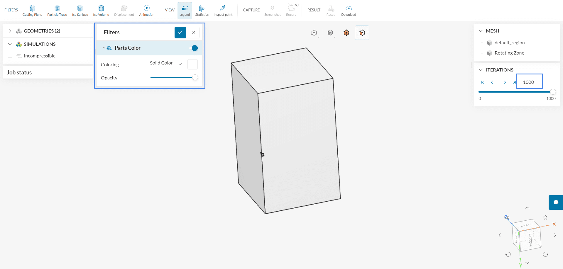
Make sure that you are at the last timestep of the simulation and no filters are applied.

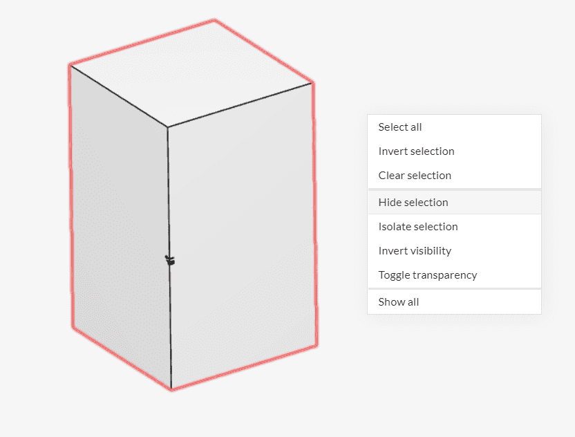
initial post-processing state — Figure 22: Make sure that the post-processor is at the last timestep and remove all predefined filters by clicking on the **‘Trash’** icon next to their name.

Hide the walls surrounding the drone by selecting them, right-clicking on the post-processor, and choosing ‘Hide selection’.

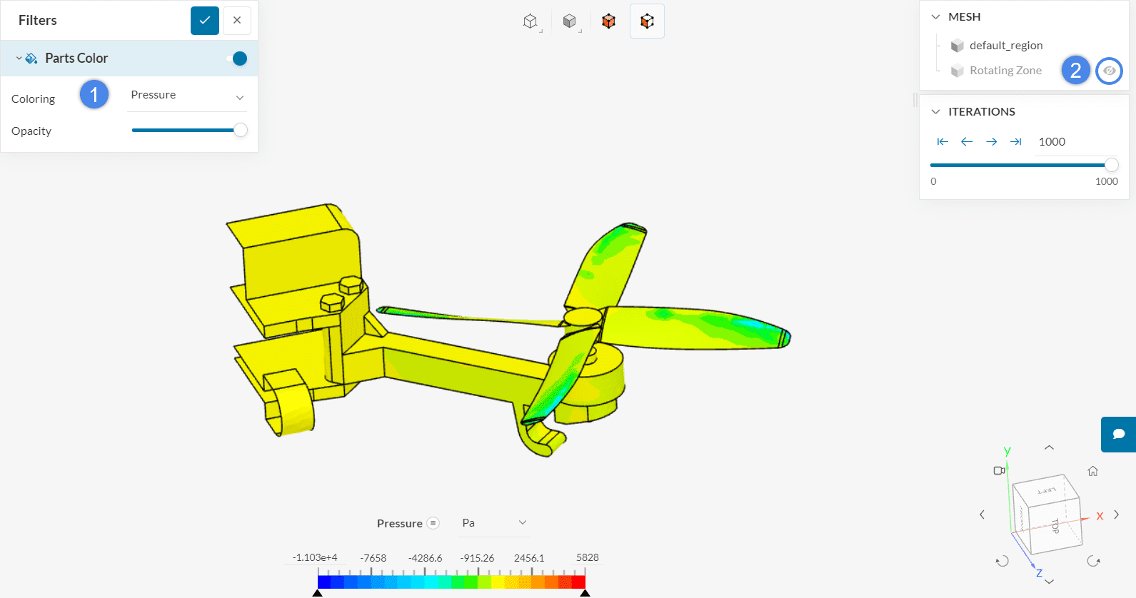
how to hide selections in simscale post-processor — Figure 23: Select the walls surrounding the drone, right-click on the mouse, and select **‘Hide selection’** to hide the walls.

Change the Coloring to ‘Pressure’ in for the Coloring of the Parts Color to show the pressure distribution on the drone. To improve the visualization, you can also hide the Rotating Zone volume by clicking on the ‘eye’ icon.

analyzing pressure levels around the blades of a propeller — Figure 24: In the *Filters* panel, change the *Coloring* to **‘Pressure’**.

The scale range is automatically set to the minimum and maximum pressure values in the domain. You can adjust the scale range to more representative bounds if required.

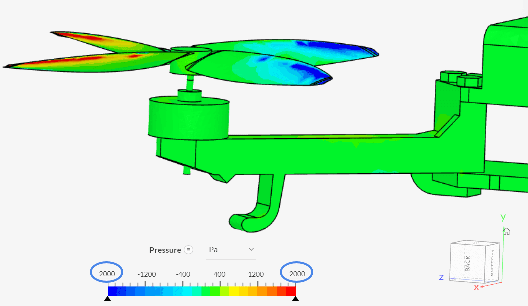
pressure distribution on the surfaces of the drone — Figure 25: Pressure distribution on the surface of the drone ranging from -2000 to 2000 \(Pa\). The bottom surfaces of the propeller and the drone arm are high-pressure zones.

As you can see from Figure 25, the highest pressures are on the bottom of the blades, which is due to the air pushed down by the propellers. Since the upper part of the blades experiences low-pressure levels, this generates a lift force, countering gravity.

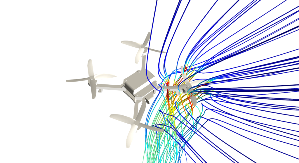
5.2 Particle Traces

We will continue showing the airflow through the propellers of the drone by using streamlines. See the steps below to create them:

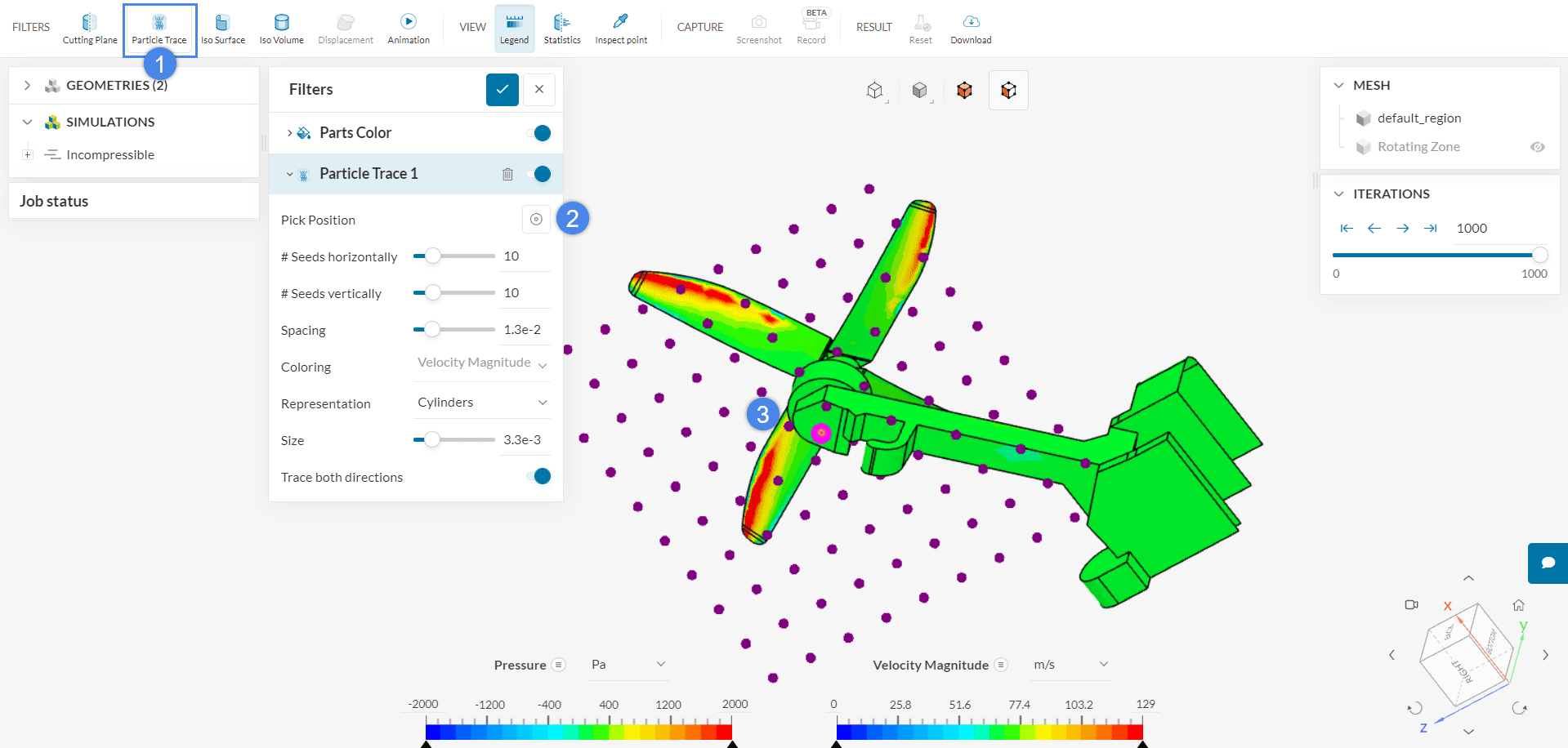
how to select particle traces in simscale post processor — Figure 26: Select **‘Particle Trace’** from the *Filters* panel.

Select a ‘Particle Trace’ filter from the top ribbon. This will lead to the settings for the particle trace setup
Make sure that the Pick Position icon is activated
Select the bottom of the drone

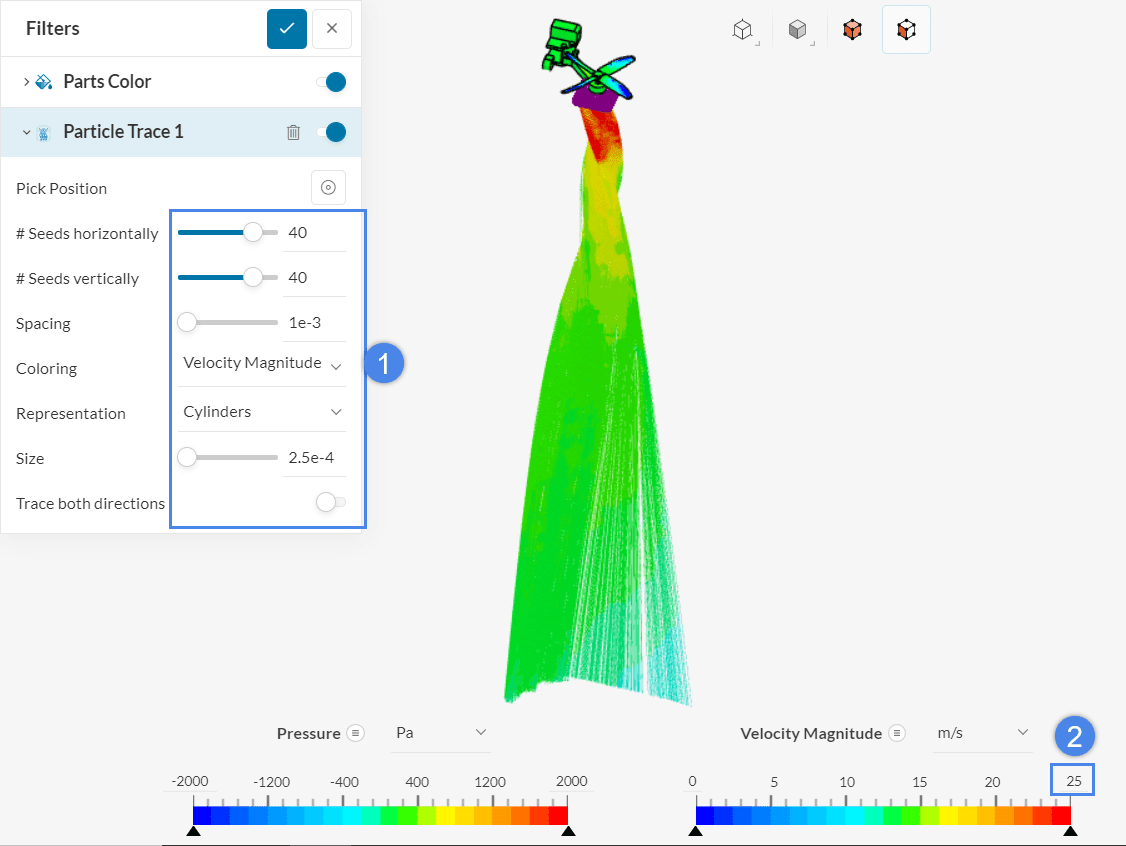
particle traces settings — Figure 27: Change the *#Seeds horizontally* and *#Seeds vertically* to **’40’**, so that there are 40 origin points vertically and horizontally. the *Spacing* and *Sizing* to **‘1e-3’**.

Next, configure the streamlines so that they are more representative. Change the #Seeds horizontally and #Seeds vertically to ’40’, so that there are 40 origin points vertically and horizontally. Change the Spacing and Sizing to ‘1e-3’ and ‘2.5e-4’, respectively.

To observe only the streamlines downstream from the drone, you can disable Trace both directions. Furthermore, adjust the upper bound of Velocity Magnitude to ’25’ \(m/s\) to make the visualization more representative.

After creating the traces, it is possible to animate them with an ‘Animation’ filter:

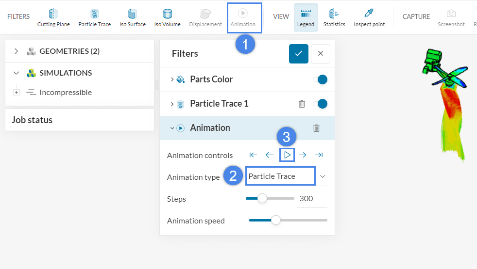
animation for particle traces — Figure 28: Velocity streamlines through the drone ranging from 0 to 25 \(m/s\)

Create an ‘Animation’ filter
Make sure that the Animation type is ‘Particle Trace’
Set the animation to run

The resulting animation looks like the video below:

drone gif animation streamlines — Animation 1: Particle trace animation in the SimScale post-processor

From the animation above, it can be seen that the flow velocity accelerates when going through the drone and creates a swirl due to the rotating movement of the propellers.

5.3 Cutting Plane

To better comprehend the velocity contours around the blades, create a cutting plane by following the steps below:

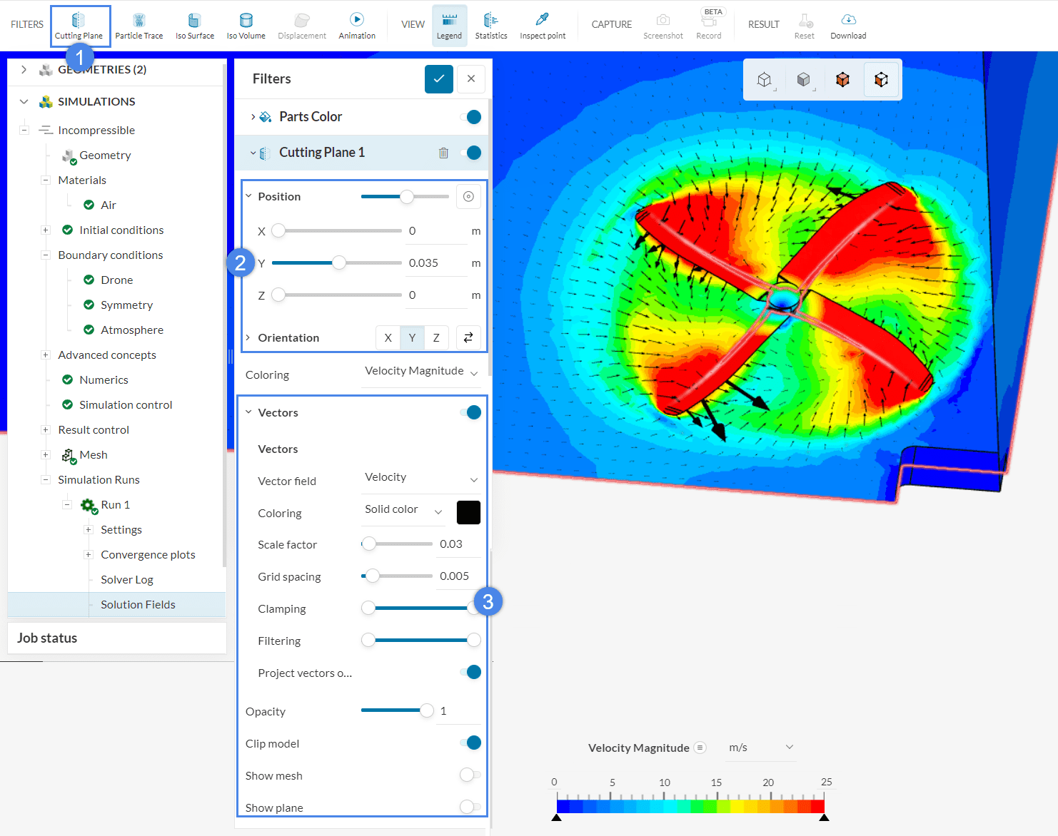
first step to creating a cutting plane — Figure 29: Select **‘Cutting Plane’** after clicking the **‘Add Filter’** button in the *Filters* panel.

Select a ‘Cutting Plane’ from the top ribbon. This will open a window with settings
Change the Position to 0 meters, 0.035 meters, and 0 meters in x, y, and z. Furthermore, change the Orientation to the y-axis
Enable the Vectors slider and change the Coloring of the vectors to a black ‘Solid color’. The Scale factor of the vectors should be ‘0.03’ with a Grid Spacing of ‘0.005’. Project the vectors onto the plane by enabling Project vectors onto Plane

From Figure 29, we can see that the velocity is higher within the propeller rotating zone. Air being pushed towards the propeller center can also be observed as a result of pressure difference and it moves in rotation according to the movement of the propellers.

You can analyze your results further with the SimScale post-processor. Have a look at our post-processing guide to learn how to use the post-processor.

Congratulations! You finished the drone with a rotating zone tutorial!

Have a look at the finished project

Note

If you have questions or suggestions, please reach out either via the forum or contact us directly.

Last updated: September 28th, 2023

Did this article solve your issue?

How can we do better?

We appreciate and value your feedback.