Documentation
Radiation is defined as the transfer of energy using electromagnetic waves. When these waves interact with any type of matter, they become heat. All bodies with a temperature greater than absolute zero emit radiation, and in contrast to conduction or convection, this radiation behavior phenomenon requires no medium.
In SimScale, radiation is available for Convective Heat Transfer, Conjugate Heat Transfer, and Conjugate Heat Transfer (IBM) analysis types and can be activated by toggling on Radiation in the global settings. As a result, you should be able to set radiative behavior, emissivity, additional radiative source, and the far-field temperature while assigning the boundary conditions, and the transparent behavior of a solid volume, can be specified under solid material assignments.
Two radiation models are used in SimScale. The first model is the Diffuse View Factors Model, which calculates the amount of radiation emitted or absorbed by a surface. The second model is the Discrete Ordinates Model, commonly referred to as DOM, which is a numerical method used to solve the radiative transfer equation.
The Diffuse View Factors model can be applied to a wide range of engineering applications where accurate radiation modeling is required. It is relatively simple to implement and use, as it mainly involves calculating view factors between surfaces and performing simplified radiation exchange calculations based on the view factors.
The different surfaces of the model will exchange heat between them, and they will also provide or subtract heat from the adjacent fluid. Coupling of both convection and radiation will be achieved once the simulation converges.
The Diffuse View Factors model is generally computationally less expensive compared to other radiation methods, especially for simulations involving simpler geometries and diffuse surface characteristics. Since it does not require solving transport equations for radiative intensity in discrete directions, it can be more efficient for certain types of simulations. In SimScale, this method is restricted to the Convective Heat Transfer solver.
The Discrete Ordinates Model (DOM) is a numerical method widely used in Computational Fluid Dynamics (CFD). The method was first proposed by Chandrasekhar (1960)\(^1\) and developed to analyze and simulate the process of thermal radiation propagation through participating media such as gases and liquids. Unlike the Diffuse View Factors model, DOM will solve the Radiative Transfer Equation (RTE), which describes the propagation of thermal radiation.
The Radiative Transfer Equation (RTE) is a five-dimensional integro-differential equation, with three spatial and two directional coordinates. This equation has a structure and function similar to the flow governing equations, as it mathematically describes the transport of radiant energy and the phenomena intrinsic to this process, such as absorption, emission, and scattering, which affect the radiation propagation in a medium.
The Radiative Transfer Equation (RTE) is given by\(^2\):
$$\frac{d I}{d s}=\hat{\mathbf{s}} \cdot \nabla I(\mathbf{r}, \hat{\mathbf{s}})=\kappa(\mathbf{r}) I_b(\mathbf{r})-\beta(\mathbf{r}) I(\mathbf{r}, \hat{\mathbf{s}})+\frac{\sigma_s(\mathbf{r})}{4 \pi} \int_{4 \pi} I\left(\mathbf{r}, \hat{\mathbf{s}}^{\prime}\right) \Phi\left(\mathbf{r}, \hat{\mathbf{s}}^{\prime}, \hat{\mathbf{s}}\right) d \Omega^{\prime}$$
Where, \(I\) is the radiative intensity. It represents the amount of radiant energy flowing in a specific direction per unit solid angle per unit wavelength and \(s\) is the wavelength of the radiation. \(\hat{\mathbf{s}}\) is the direction vector representing the direction of radiation propagation, and \(\mathbf{r}\) is the position vector. \(\kappa\) is the absorption coefficient and it represents the proportionality constant between the absorption of radiant energy and the radiative intensity. \(\beta\) is the scattering coefficient and it represents the proportionality constant between the scattering of radiant energy and the radiative intensity. \(\sigma_s\) is the scattering coefficient for emission and it represents the proportionality constant between the emission of radiant energy and the radiative intensity. \(dΩ_i\) represents the infinitesimal solid angle element in the emission direction.
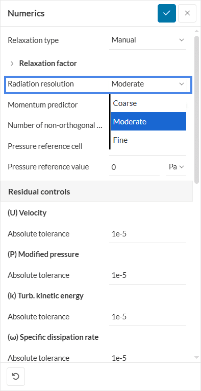
In the Discrete Ordinates Model, the RTE equation is discretized into a finite number of discrete directions or “ordinates” over which the radiative intensity is calculated. These discrete directions represent the angular dependence of radiation propagation. Each discrete direction corresponds to a specific “beam” or “ray” of radiation propagating through the medium. These directions are chosen to sufficiently sample the angular distribution of radiation within the domain being modeled. In SimScale, you can adjust the number of beam directions for your simulation using the Radiation Resolution option. This feature offers three options: Coarse, Moderate, and Fine, which correspond to 8, 32, and 72 beam directions respectively. Note that using more beam directions will increase the simulation time.
As the flow governing equations, SimScale will use the Finite Volume method to solve this set of transport equations for the radiative intensity in each discrete direction. The Conjugate Heat Transfer solver uses the Discrete Ordinates Model (DOM).
Radiative behavior specifies the relationship between the net radiative heat per unit surface area, \(Q_r\ [W/m^2]\) and the temperature of every surface, \(T_s\ [K]\). In SimScale, you can set three radiative surface behaviors, opaque, transparent and semi-transparent as well as one radiative volume behavior which is fully transparent in material assignments:
A Transparent surface establishes no relation between \(Q_r\) and \(T_s\). This means that the surface temperature remains unaffected by the net radiative heat that the surface emits or receives. This implies that \(T_s\) is determined by other heat transport means (conduction or convection) or by a boundary condition. This option is mainly applied to surfaces that are not solid, like inlets or outlets (for example, an open window).
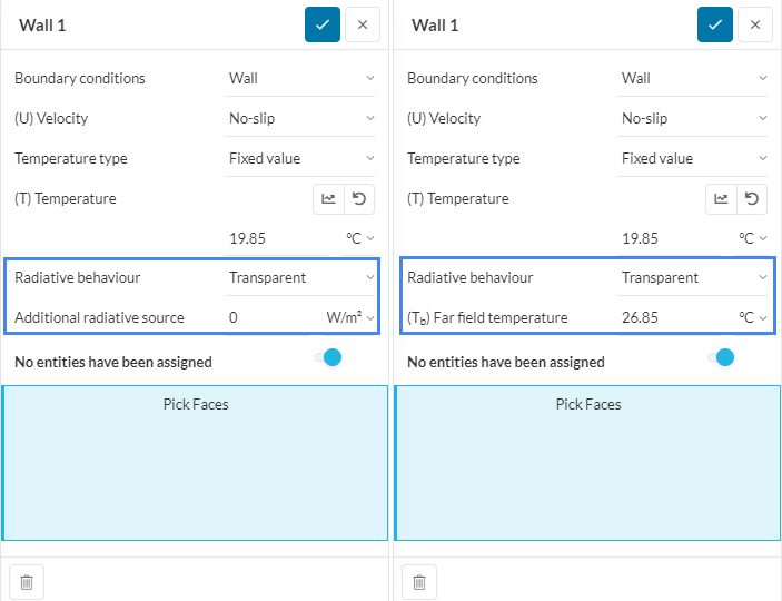
Additional Radiative Source
For convective heat transfer analysis, apart from the radiative heat interchange that the surfaces will perform, we can set an additional radiative source. This represents any additional (mainly external) source of radiation that goes through the surface and it will not heat it up. The best example is solar radiation getting into the domain through an open window.
Far Field Temperature
Available to only conjugate heat transfer analysis, far-field temperature represents the temperature of the black body in the far field needed for inclusion of radiation effects at the open boundaries. Hence, instead of mentioning the power of the radiative source you can just mention its temperature.
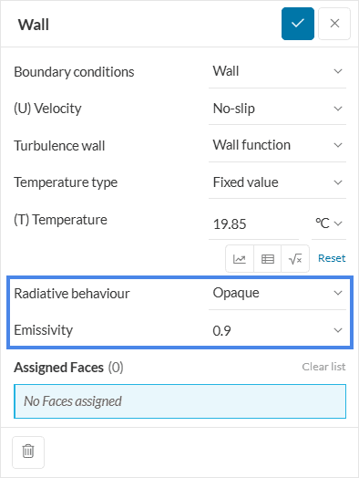
An Opaque behavior couples \(Q_r\) and \(T_s\) using the Stefan-Boltzmann law for diffuse and hemispheric radiation. Supposing two different surfaces \(S\) and \(S’\), the \(Q_r\) that \(S\) provides to \(S’\) is:
$$ Q_r(S→S’) = F. \epsilon . \sigma .(T_S – T_{S’})^4$$
Where \(F\) is the view factor between \(S\) and \(S’\), \(\sigma\) is the Stefan-Boltzmann constant (5.6696e-8 \(W /m²K\)), and \(\epsilon\) is the emissivity of the surface \(S\).
A surface that is not fully transparent is considered a semi-transparent surface. Such a surface partially absorbs, transmits, and reflects the radiation falling on it. The user needs to provide the values for the emissivity as well as transmissivity. This is only available for CHT and CHT (IBM) analysis type.
Emissivity
The emissivity depends on the material of the surface, and it measures its capability to emit radiation, otherwise known as its radiation behavior. For opaque surfaces, the default value in the Workbench is 0.9, which is a good approximation for walls made of brick or concrete.
Transmissivity
Transmissivity also depends on the material of the surface, and it measures its capability to transmit radiation. For semi-transparent surfaces, the default value in the Workbench is 0.7, which is a good approximation for stained glass windows.
While transparent surfaces only apply to boundary faces, it is also possible to define the transparent behavior of entire solid volumes. This option is available under solid material assignments for Conjugate Heat Transfer (CHT) and Conjugate Heat Transfer (IBM) analyses. In practice, this allows users to assign a solid region, such as glass with a specified thickness, as transparent to radiation while still participating in conduction and convection. A transparent solid has the following characteristics:
This behavior is fundamentally different from boundary condition settings, which are applied at surfaces to control how they interact with the radiation model. Transparent solids, on the other hand, extend this property to the bulk material itself, allowing an entire region to transmit radiation without radiative coupling to its temperature.
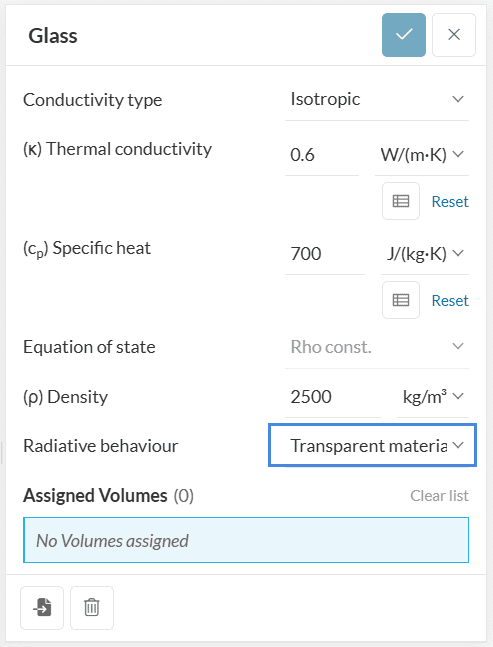
Figure 3 illustrates how such transparent solids can be defined in the Workbench, where a solid region (e.g., a glass pane) is assigned as transparent within the solid material properties. By contrast, if radiation absorption or partial transmissivity is important on surfaces (e.g., stained or coated glass, plastics, ceramics), then the semi-transparent surface behavior should be used instead, as transparent solids will not capture these effects.
For radiative heat transfer problems, further settings can be changed within the numerics, as shown in the picture below. Most importantly, the radiation resolution can be changed. This affects the discretization of the directions for which the radiative problem is solved. The settings are coarse, moderate, and fine. Increasing the radiation resolution will lead to a higher number of directions and hence improved angular discretization of the radiative problem (usually a more accurate result).
To read more about supported types of radiation and radiation behavior check out this documentation page.
References
Last updated: September 30th, 2025
We appreciate and value your feedback.
Sign up for SimScale
and start simulating now


