In this short article, you will learn to check convergence and its assessment in the SimScale Workbench.
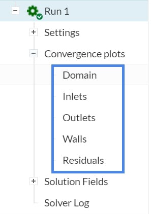
1. Check the Convergence Plots
The convergence plots section should be the first starting point to check the convergence of your simulation. These plots will help you to understand the global and local imbalances in a CFD simulation.
1.1 Check the Residuals
In an iterative solution, residuals are the solution imbalances. For numerical accuracy, you should expect residuals to be as small as possible. Usually, residuals below 1e-3 is a good starting point to move to the next check.
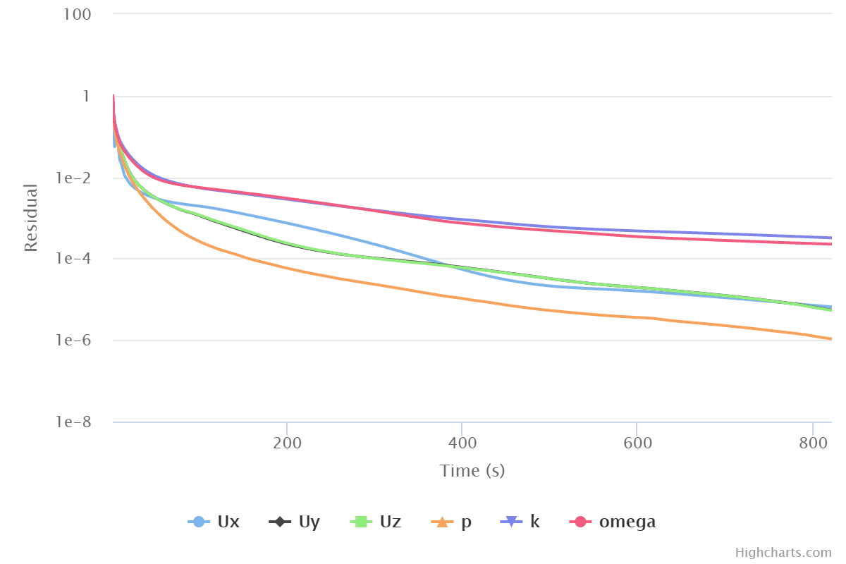
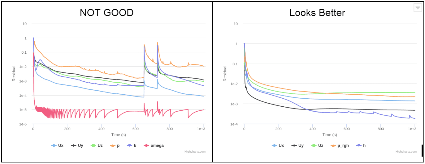
The residual plot also gives an idea regarding the stability of a solution. Observing sudden spikes shows that the solution encountered problems. The results of such simulations are not reliable.
1.2 Check the Convergence Plots for Boundary Conditions
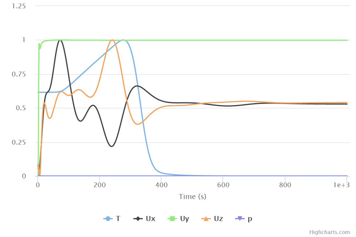
The convergence plots for boundary conditions are grouped as Domain, Inlets, Outlets, and Walls. Each convergence plot represents the average of each variable for every iteration, normalized to a range from 0 to 1. If your residual plot shows a bad convergence and you wonder why, you can check convergence plots for the domain, inlets, outlets, and walls. Let’s check the following example:
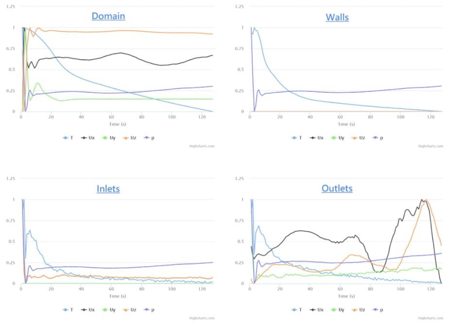
The first picture presents convergence for the whole domain. U_x (velocity in x-axis) seems slightly fluctuating. T (temperature) is stable but keeps reducing. This does not show any stability issue but only shows that the temperature inside the domain is not converged yet. Consequently, more iterations are needed. Other parameters look stable.
Walls and Inlets convergence plots also look good. Small fluctuations at the inlets can be ignored.
Outlets convergence plot shows some serious issues. High fluctuations are observed in pressure and velocity values. This is a clear indicator that boundary conditions or the mesh quality might be responsible for numerical issues at the outlets.
Let’s check the Outlets convergence plot of a successful simulation. The example below shows that the flow at the outlets was initially unstable, but after approximately 800 iterations, the stability is achieved:
2. Check the Result Control Items
In an iterative solution, the calculation process starts with initial estimations of quantities (pressure, velocity, temperature, etc.). In every iteration, quantities are updated with respect to the previous iteration results. In a converged steady state solution, one should expect to see that those quantities come to a level and don’t change anymore.
In SimScale, the best way to check the convergence of a quantity of interest is to use result control items. You can see more information about the result control on this page.
The following graph belongs to a pressure drop simulation. The quantity of interest for this simulation is the pressure difference. First, the simulation was performed for 300 iterations, and area average pressure values at the inlet and outlet were re calculated:
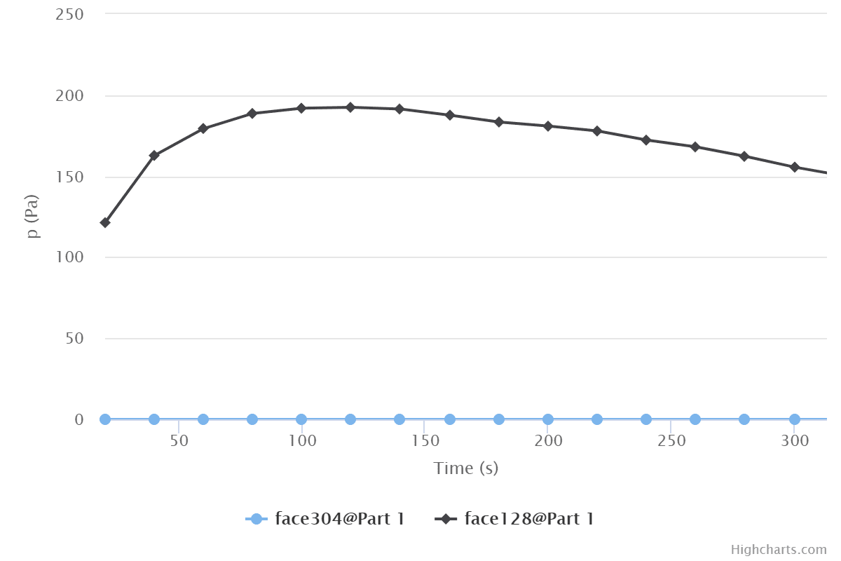
While the pressure on one surface is stable at 0 \(Pa\) (outlet), the other one is close to 150 \(Pa\) and yet is not converged. The result cannot be trusted and further iterations are needed until the quantity is converged.
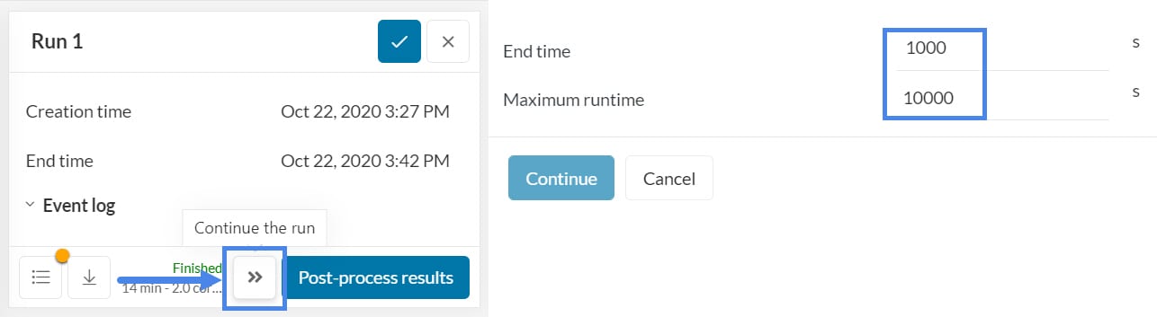
Just click on the simulation run. You will see the “Continue to run” icon. In this example, we ran the simulation until 1000 iterations.
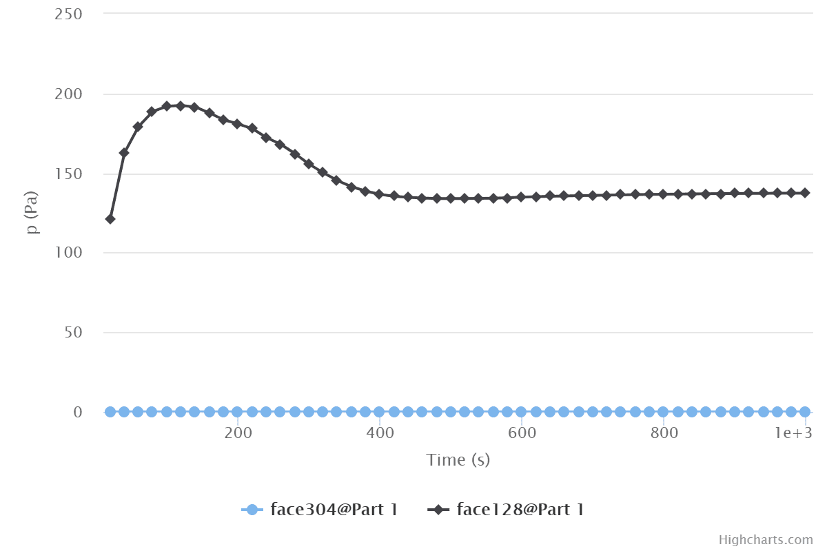
Results show that the inlet pressure value is converged around 500 iterations. Both convergence plot, as well as the plot for the quantity of interest, are converged. Finally, you can monitor the solution fields to check if the results look realistic.


