Compressible Flow vs Incompressible Flow
In this article, we explore the differences between compressible flow and incompressible flow analyses through basic definitions, distinguishing criteria, equations, and applications. But first, what is a flow?
A flow is a movement of fluids (liquids, vapors, and gases) that passes through a given point per unit time. Fluid flow is a part of fluid mechanics that deals with the dynamics of fluids. This movement is the result of different unbalanced forces and continues until a balance between the applied forces is achieved. A simple example would be a waterfall falling from a height due to gravity.
Types of Flows
In fluid mechanics, flows can be classified into various categories based on the nature of the flow. The different types of fluid flows are:
- Steady and Unsteady
- Uniform and Non-uniform
- Laminar and Turbulent
- Compressible and Incompressible
- Rotational and Irrotational
- …and many more.
Here, we’ll focus on what differentiates compressible flow from incompressible flow.
Difference between Compressible and Incompressible Flow
In a compressible flow, the density of the fluid does not remain constant.
$$ \rho \neq constant \tag{1}$$
On the other hand, incompressible flows are defined as those in which the density of the fluid remains constant.
$$ \rho = constant \tag{2}$$
Thus, in the mechanics of materials terminology, shear forces on the incompressible fluid due to viscosity or external body forces do not cause changes in density during flow.
Compressibility and Mach Number
Due to the malleable structure of fluids, the compressibility of fluid particles is a significant issue. In reality, all fluids are compressible by nature. Despite the fact that all types of fluid flows are compressible in various ranges of molecular structures, most of them can be assumed incompressible since the density changes are negligible.
However, high-speed flows where the velocity is beyond a critical limit cannot be assumed incompressible. This is determined by the Mach Number. Mach Number is a dimensionless number that compares the flow velocity with the speed of sound in the surrounding medium. It is calculated as follows:
$$ Ma=\frac{V}{a}\ \tag{3}$$
where \(Ma\) is the Mach number, \(V\) is the velocity of flow, and \(a\) is the speed of sound in the flow medium and is a function of its temperature.
- When Mach number is less than 0.3, the flow can be considered incompressible.
- When Mach number is larger than 0.3 – i.e., high-speed flows – the change in density is not negligible, and the flow is considered compressible.
In the air at 20 \(°C\) and 1 \(atm\) (101,325 \(Pa\)), sound velocity is approximately 340 \(m/s\). Therefore, Mach number 0.3 corresponds to a flow velocity of approximately 100 \(m/s\). For instance, if the velocity of a car is higher than 100 \(m/s\), the suitable approach to conducting credible numerical analysis is the compressible flow.
Density as a Criterion for Classification of Flows
A common criterion for classifying compressible and incompressible flows is when the density change is 5% or less, the flow is considered incompressible. When the density is greater than 5%, the flow is compressible. A 5% change in density is equivalent to a Mach number of about 0.3.
The criterion limit for density change can be arbitrary. If the threshold is set to a strict 1%, then Mach number would roughly be 0.14, and the flow velocity would be about 50 \(m/s\). Keep in mind that even when the flow velocity is the same, Mach number can change because sound velocity varies with temperature and pressure.
On the other hand, the density of a liquid, such as water, changes very little. The speed of sound in water is higher than that in gas. For instance, sound propagation through water is around 1481 \(m/s\) at 20 \(°C\) and 1 \(atm\). As a result, a liquid is commonly referred to as an incompressible fluid.
Governing Equations for Compressible Flow and Incompressible Flow
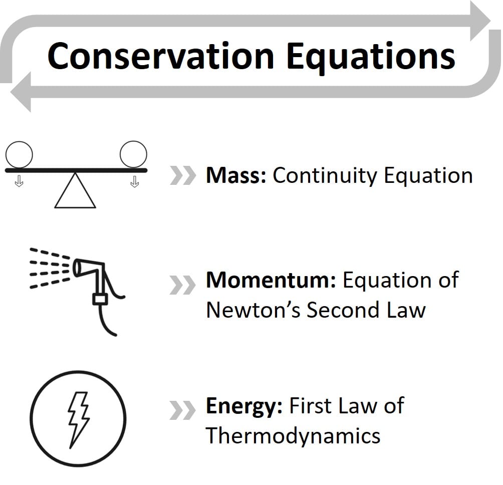
The equations that govern the fluid flow are based on the conservation laws of a fluid’s physical properties. The basic equations are the three laws of conservation1:
- Conservation of Mass: Continuity Equation
- Conservation of Momentum: Navier Stokes Equation
- Conservation of Energy: First Law of Thermodynamics or Energy Equation
Continuity Equation
The equation for the Conservation of Mass is specified as:
$$ \frac{Dρ}{Dt} +\rho (\nabla \cdot \vec{v}) =0 \tag{4}$$
where \(\rho\) is the density, \(\vec{v}\) the velocity and \(\nabla\) the gradient operator.
$$ \vec{\nabla} = \vec{i} \frac{\partial}{\partial x} + \vec{j} \frac{\partial}{\partial y} + \vec{k} \frac{\partial}{\partial z} \tag{5}$$
For incompressible fluids where the density is constant, the continuity equation reduces to:
$$ \frac{D\rho}{Dt} = 0 \rightarrow \nabla \cdot \vec{v} = \frac{\partial u}{\partial x} + \frac{\partial v}{\partial y} + \frac{\partial w}{\partial z} = 0 \tag{6}$$
Navier-Stokes Equation
Conservation of Momentum which can be referred to as the Navier-Stokes Equation is given by:
$$ \overbrace{\frac{\partial}{\partial t} (\rho \vec{v})}^{I} + \overbrace{\nabla \cdot (\rho \vec{v} \vec{v})}^{II}= \overbrace{-\nabla p}^{III} + \overbrace{\nabla \cdot \left(\overline{\overline{\tau}}\right)}^{IV} + \overbrace{\rho \vec{g}}^{V} \tag{7}$$
where \(p\) is static pressure, \(\overline{\overline{\tau}}\) is viscous stress tensor and \(\rho \vec{g}\) is the gravitational force per unit volume. Here, the Roman numerals denote:
I: Local change with time
II: Momentum convection
III: Surface force
IV: Diffusion term
V: Mass force
Viscous stress tensor \(\overline{\overline{\tau}}\) can be specified as below in accordance with Stoke’s Hypothesis:
$$ \tau_{ij} = \mu \frac{\partial v_i}{\partial x_j} + \frac{\partial v_j}{\partial x_i} – \frac{2}{3}(\nabla \cdot \vec{v}) \delta_{ij} \tag{8}$$
If the fluid is assumed to be incompressible with constant viscosity coefficient \(\mu\), the Navier-Stokes equation simplifies to:
$$ \rho \frac{D\vec{v}}{Dt} = -\nabla p + \mu \nabla^2 \vec{v} + \rho \vec{g} \tag{9}$$
Energy Equation
The conservation of mass and momentum equations are not enough to represent a fluid flow. An additional enthalpy equation from thermodynamics is required that includes a dissipation term and accounts for temperature changes during flow when heat or any other energy exchange is involved.
Convective and conjugate heat transfer simulations involve thermal energy transfers for accurate CFD analysis. Stress-strain relations for compressible fluids can further complicate equations of compressible flow.
For more information on the governing equations please have a look at the following SimWiki article:
Applications
Incompressible Flow
Incompressible flow modeling is used for a large number of applications in CFD. Listed below are some common applications:
Flow through valves and water turbines
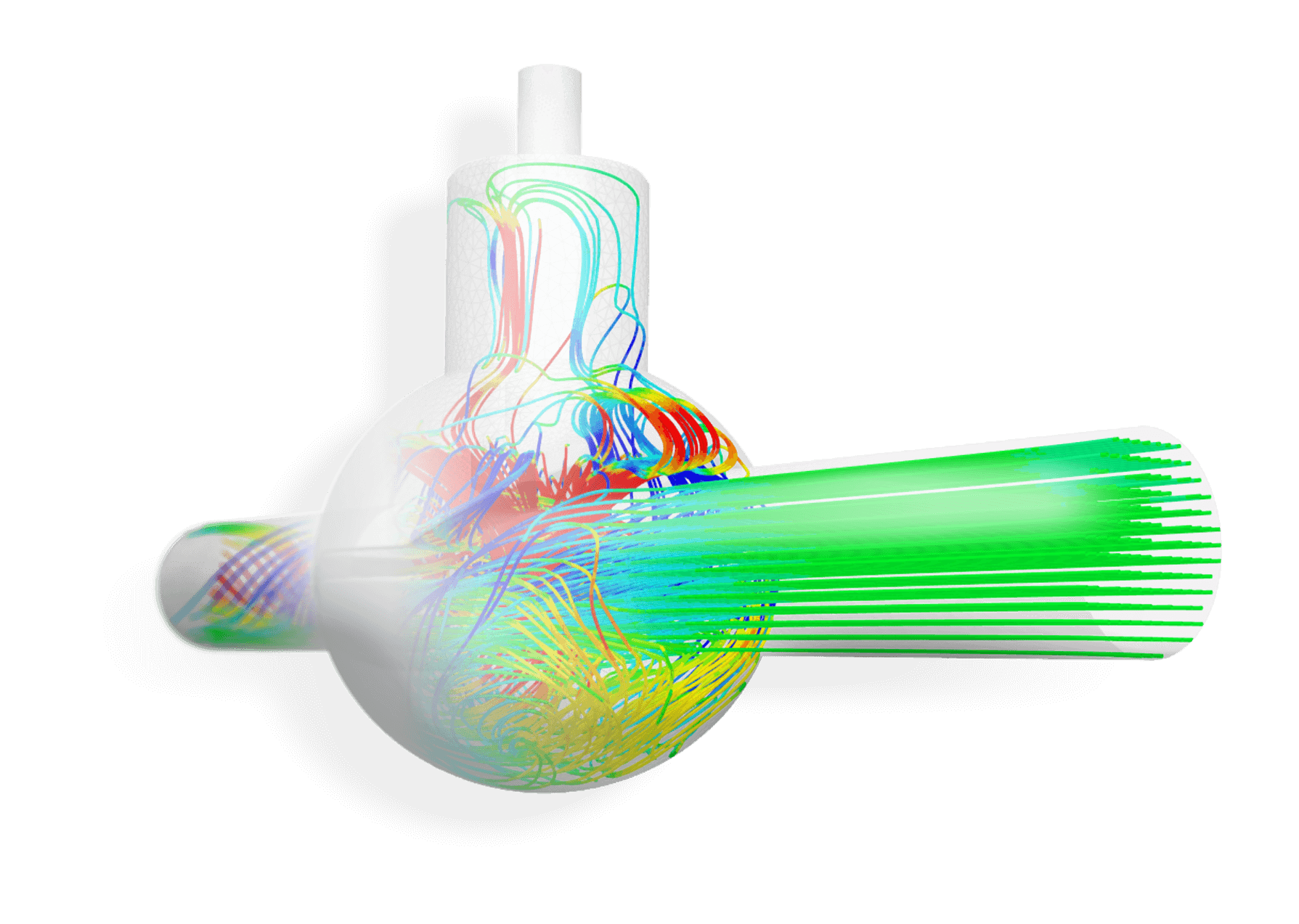
Understanding the pressure differences between inlet and outlet for a range of flow rates can provide optimum working conditions for the highest efficiency. This helps in extending the life of casualties.
Ventilation in a parking lot
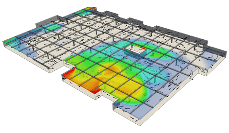
Parking spaces can get pretty packed at peak times which is where the presence of HVAC systems like exhaust fans becomes crucial. Through CFD simulations, passive entities like smoke coming out of the car can be detected and tracked to understand the safety standard in such congested spaces
Aerodynamics of vehicles
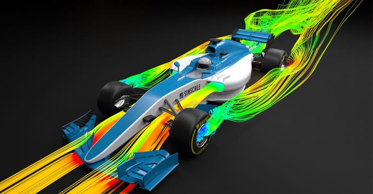
Incompressible flow analysis is extremely common in the aerodynamics/hydrodynamics of vehicles where the Mach number is low \(Ma\) < 0.3. Also, for extreme cases like aerodynamics in Formula 1 racing (F1), the velocity is not high enough to make the compressibility relevant (the record velocity in F1 is 372.5 \(km/h\) 10 corresponding to \(Ma\) = 0.29 at \(T\)= 40 \(°C\)).
Compressible Flow
Numerous engineering applications that involve high-speed flows and/or flows with significant pressure differences are compressible in nature.
Aeroplane Wing analysis
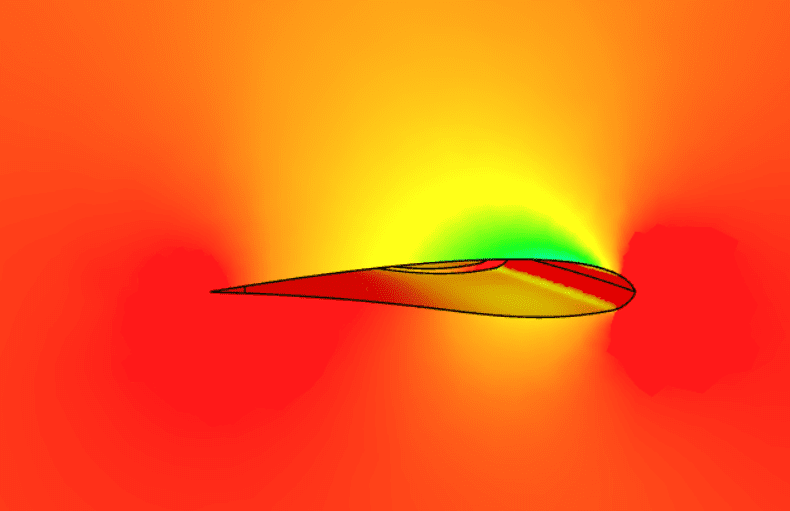
Most commercial airlines fly between the speed range of 0.6-0.9 Mach which lies in the compressible analysis category. Aerodynamic development of wing designs is boosted with CFD simulations accurately predicting the turbulence and vortices developed around the wing
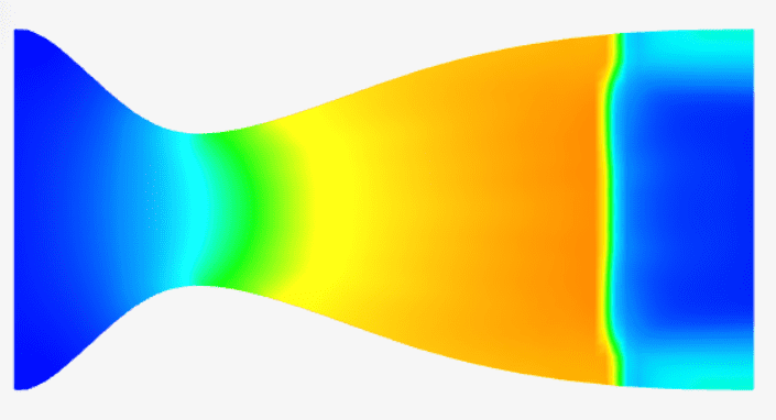
In supersonic (1.2-5 Mach) and hypersonic (5-10 Mach) ranges, shocks are formed, which can also be captured in the simulation using compressible flow analysis.
Gas and Steam turbines
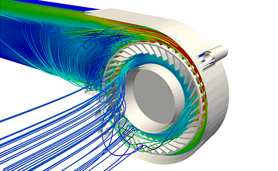
Manufacturers/Scientists provide data curves for turbomachinery that describe the relationship between static pressure, power requirement, rotational speed, and efficiency values per-flow rate conditions. The experimental tests for the design of rotating parts are so intricate and expensive, that simulation data is necessary to help engineers make decisions early in the design process, like achieving the desired flow rate/cooling conditions, without having to practically deal with high-pressure and temperature situations.
Internal Combustion Engines
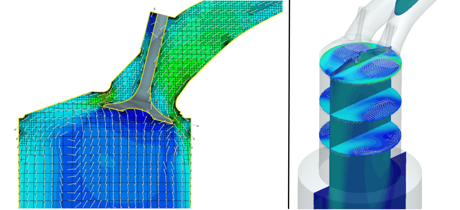
CFD modeling of IC engines can evaluate the combustion of new fuel and air inlets and reduce emissions at a lower cost of analysis. The development of contemporary internal combustion (IC) engines, depends on CFD simulations as they can offer suggestions for additional advancements in engine technology.
Furthermore, simulations can be used to examine flow in situations and locations where measurements are problematic due to factors like high temperatures and pressures, for example.
CFD Simulation in SimScale
SimScale’s CFD software can analyze a range of problems related to laminar and turbulent flows, incompressible and compressible fluids, multiphase flows, and much more. With everything 100% in the web browser, the barriers of limited computing power, accessibility, and high costs are eliminated.
There are numerous analysis types to choose from where one can decide whether to include compressibility effects. Standalone Incompressible and Compressible flow analysis types are also available.

SimScale’s CFD simulation software can solve complex flow equations with accurate numerical methods, powerful turbulence models, and complex CAD handling robust solvers, by offering everything under one tool.
Tutorials and User Guides
You can find several SimScale tutorials and user manuals here, which should cover user manuals for particular industries and the most typical use cases:
References
- Frank M. White, Viscous Fluid Flow, McGraw-Hill Mechanical Engineering, 3rd Edition, ISBN-10: 0072402318
Last updated: August 11th, 2023
Did this article solve your issue?
How can we do better?
We appreciate and value your feedback.
What's Next
What is Lift, Drag, and Pitch?

