Documentation
This tutorial will provide step-by-step guidance on how to set up a contamination control simulation inside a car park.
This tutorial will teach you how to do the following:
This tutorial will follow the usual SimScale workflow:
First, you should import this project into your Workbench.
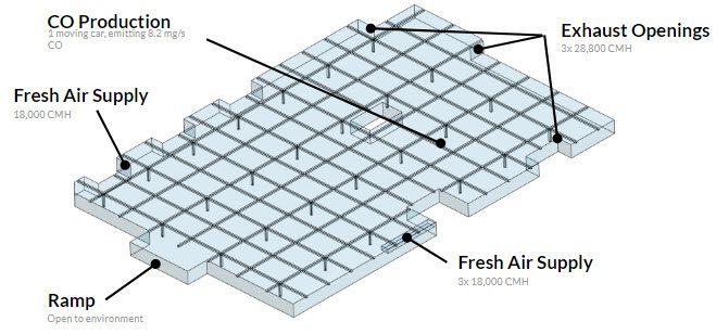
By importing the tutorial project, a new project containing the car park geometry can be seen:
In the translucent render mode, you can see the jet fans and the car has been included in the model. This will make the simulation setup process easier because we will only need to select these bodies later. You can also notice this fact by examining the individual components under the scene tree on the right of the Workbench.
You can follow the steps below to create your simulation:
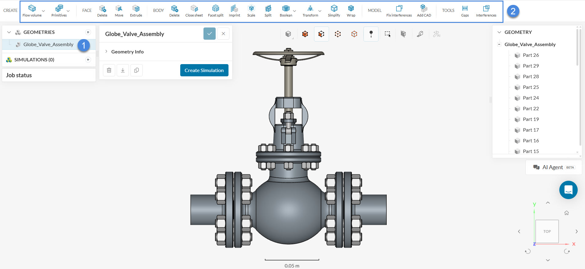
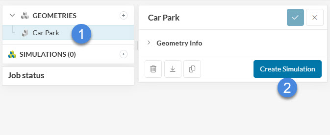
First of all, to create a new simulation, click on the ‘+’ button next to Simulations in the simulation tree or the ‘Create Simulation’ button on the geometry panel.
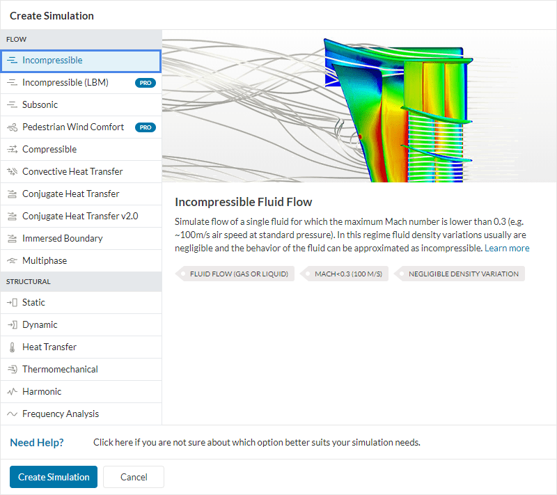
Next, select the ‘Incompressible’ analysis type and click on ‘Create Simulation’.
Doing so creates a new simulation tree, like shown below:
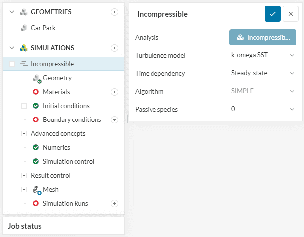
All setup steps that are already sufficient for initializing the simulation are highlighted with a green checkmark. Steps that require some user input are shown with a red circle and those that have a blue circle indicate optional settings.
In this section, we will be defining the physics of our model for the car park contamination simulation.
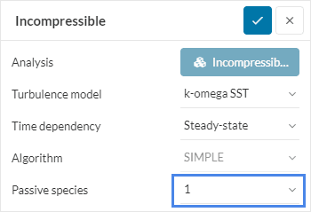
To define a contaminant for our car park contamination simulation, we will need to define a passive species in our simulation. This is done by following the steps below:
Read more:
You can find more information and instructions on passive species modeling below:
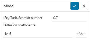
A scalar transport simulation is highly dependent on two aspects:
You can change these values in the Model settings panel in your simulation tree, but for this simulation, we will use the default values.
Air will be assigned as the simulated material in the simulation. To define this, click on the ‘+’ button next to Materials, which opens the SimScale material library:
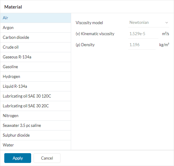
Select ‘Air’ and confirm your choice by hitting ‘Apply’. A dialog box showing all the physical parameters of the selected material will show up:
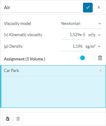
We will select ‘Car Park’ as the fluid region of the simulation (from the scene tree on the right) and confirm the operation by hitting the check box on the top right of the material dialog box.
You can also just select any material from the library, and change its name and properties to define a custom material.
In this section, you are able to modify the initial conditions of the simulation. This simulation is not time-dependent, which means that it will not affect your results, whatever you define here. However, if you already have a correct guess about the end result, adding it here will stabilize the simulation and help the solver to converge faster.
In this case also if you don’t know the end result, just leave the initial conditions at their default values.
This simulation will use three boundary conditions:
Saved Selections
To make the further boundary condition assignment easier, the faces belonging to the same boundary condition are grouped within a Saved Selection. You can find them on the right side of the Workbench in the scene tree under Saved Selections.
The following picture shows how to create them, in case you want to do them yourself.
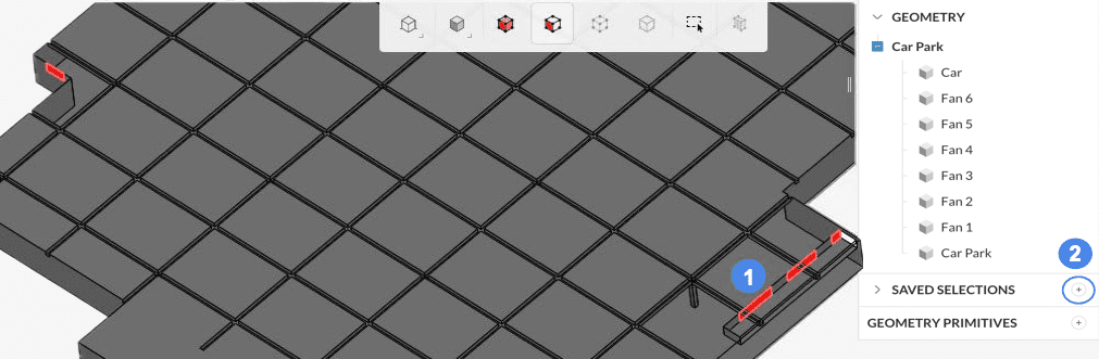
Now go ahead and create another set for the outlets.
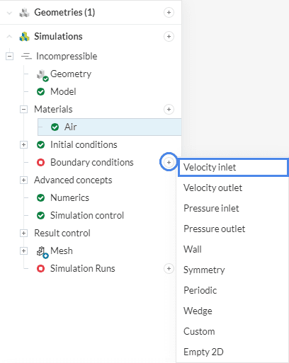
To define the boundary conditions, click on ‘+’ next to Boundary conditions, which opens the boundary condition library, as shown in the picture below:
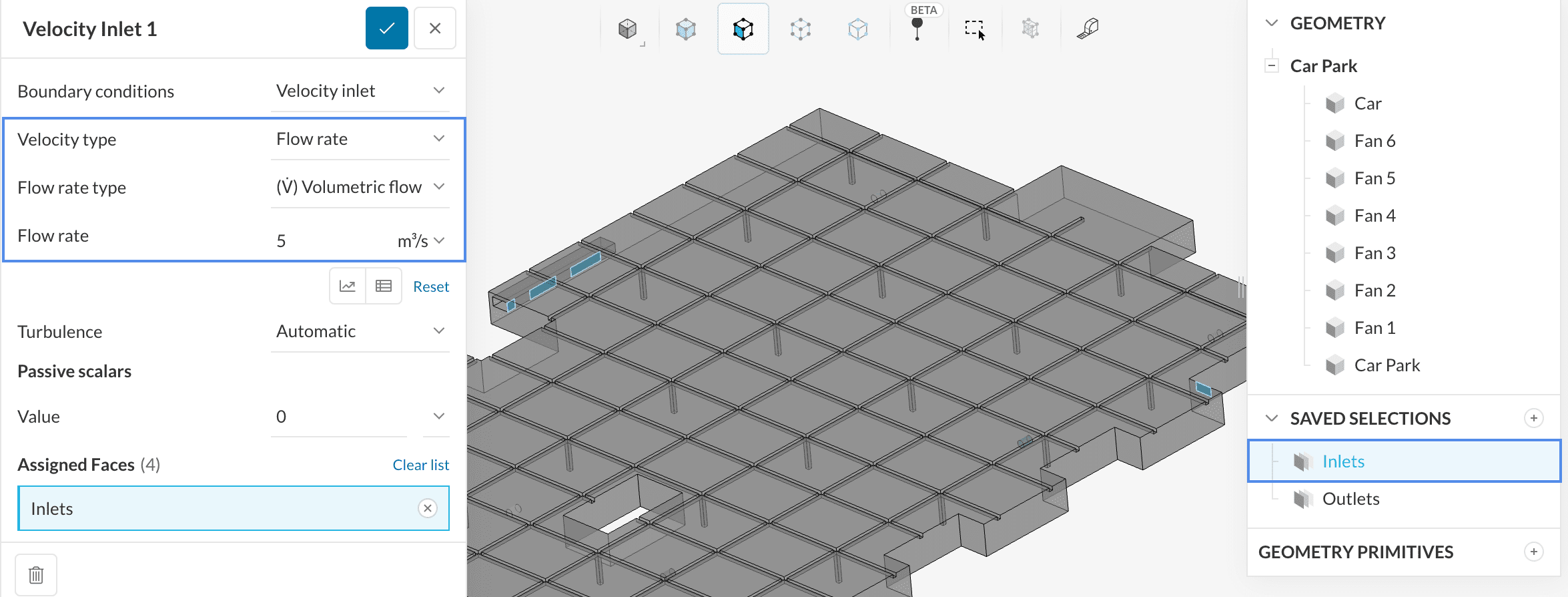
To define the inlets, please create a new Velocity inlet boundary condition, and assign the properties according to the following picture.
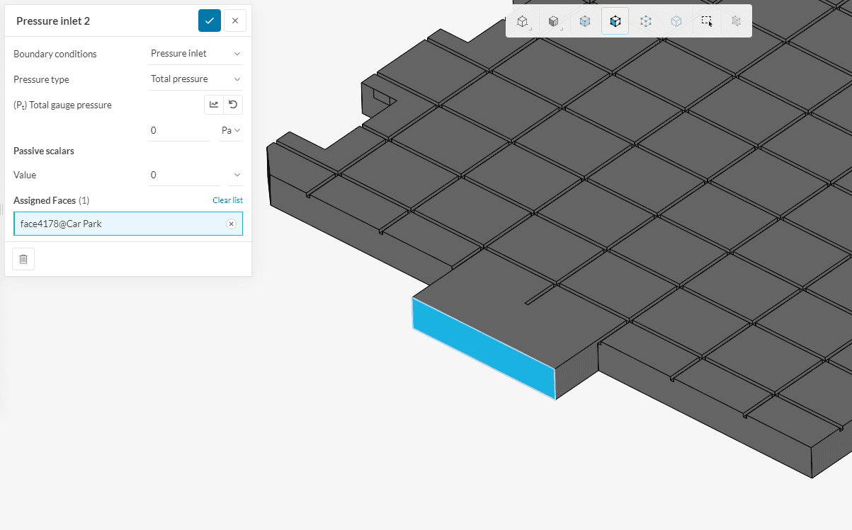
For the remaining inlet, we will define a Pressure inlet. Therefore follow the steps from Figure 14. Define the settings as presented in the picture below:
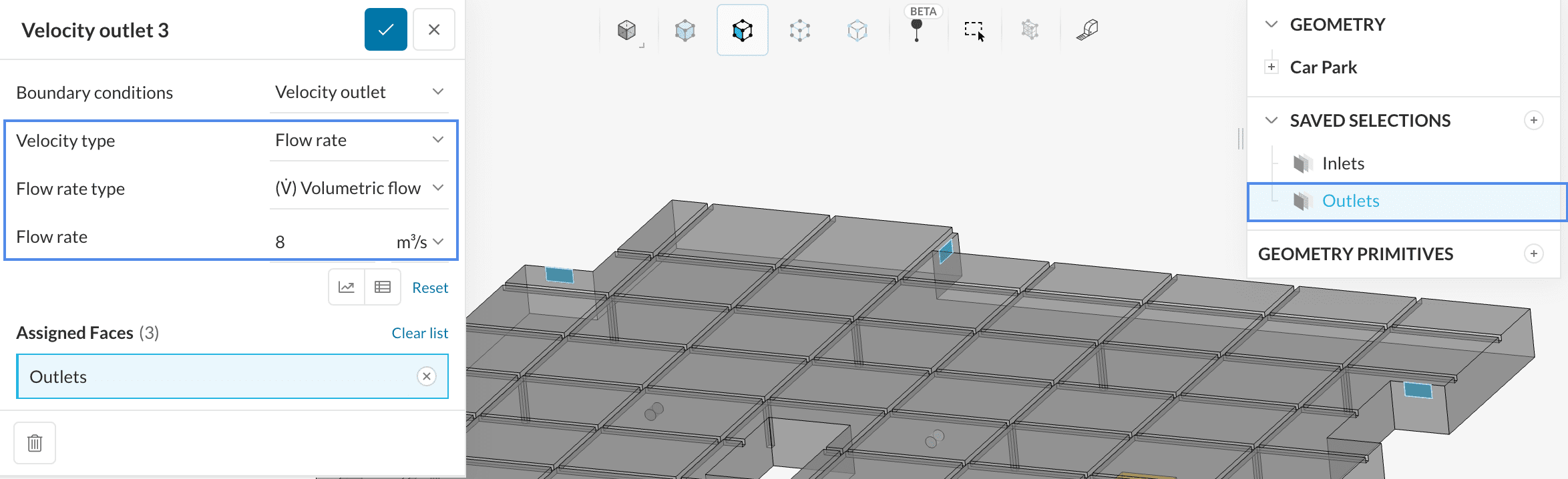
Finally, we need to define the location of the outlets. Therefore, create a Velocity outlet according to Figure 10 and define it as presented in the picture below:
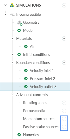
Under Advanced concepts, we will define the setup for Momentum sources to model the fans for the ventilation in the car park and the CO concentrations by defining a Passive scalar source. The jet fans and the car has been included in the model, so there is no need to create any new geometry.
Click on ‘Advanced concepts’ and hit the ‘+’ button right next to the respective item, like presented in the picture below:
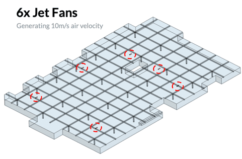
We will also model the jet fans installed in the car park as the mitigation method to circulate CO out of the car park. To do this, create a Momentum Source by hitting the ‘+’ button:
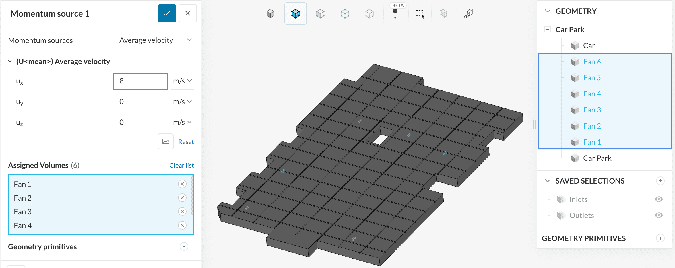
Next, we will assign the average velocity of the fans which is 8 \(m/s\) in the X-direction and select all the Fan parts in the model (again, use the scene tree).
We will set a velocity for the CO coming out of the car by following the similar steps above but instead of selecting the fans, we will use the Car as the momentum source.
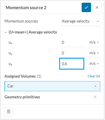
The velocity of the CO emitted by the car will be 0.8 \(m/s\) in the z-direction.
Create a Passive scalar source like demonstrated in the Figure 17 above, then define the setup according to the following figure:
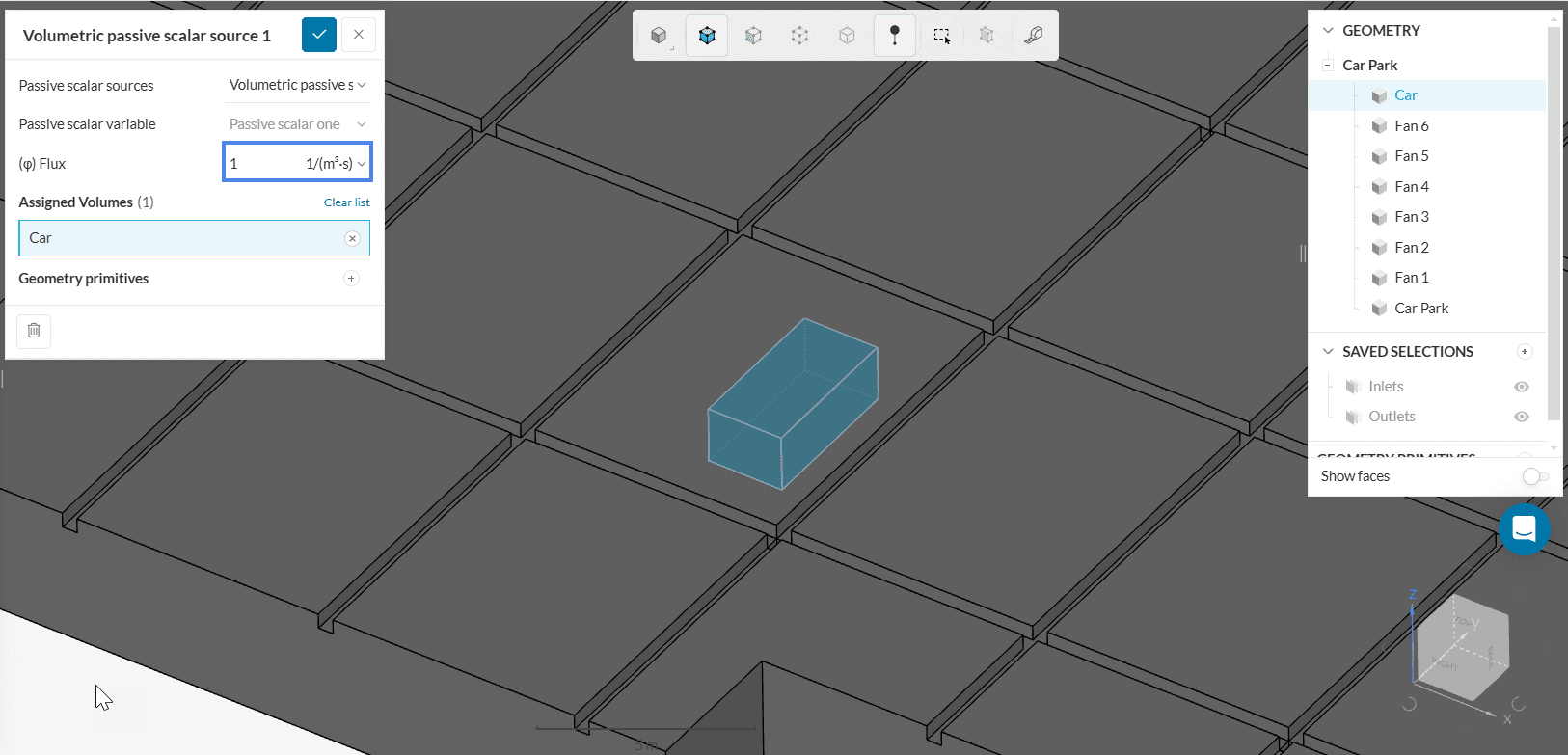
Confirm the definition by hitting the check button on the top right of the panel.
You can find definitions and details about the passive scalar flux in this documentation page.
The tree item Numerics enables to control the numerical settings for the solver. The default values are fine for most simulations, however, experts can define whatever numerical settings they want.
For this tutorial, the default values are good enough.
The next important tree item is Simulation control which allows steering the overall simulation settings. For this car park contamination simulation we will increase the End time to ‘1500’ seconds.

Convergence
This tutorial converges enough within 1500 iterations. In case you are not satisfied increase the End time.
In order for you to get an accurate result, a good mesh is necessary. However, the finer the mesh the more core hours will be consumed. It is best to start from a coarse mesh and increase the fineness level if necessary. You can create your mesh by clicking ‘Mesh’ in the simulation tree. This simulation utilizes the Standard meshing algorithm. You can keep all parameters with their default values.
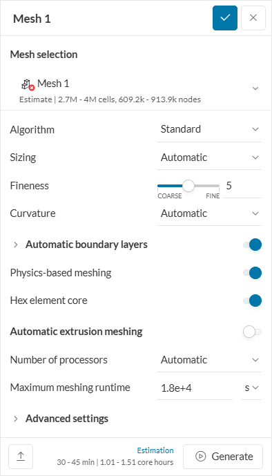
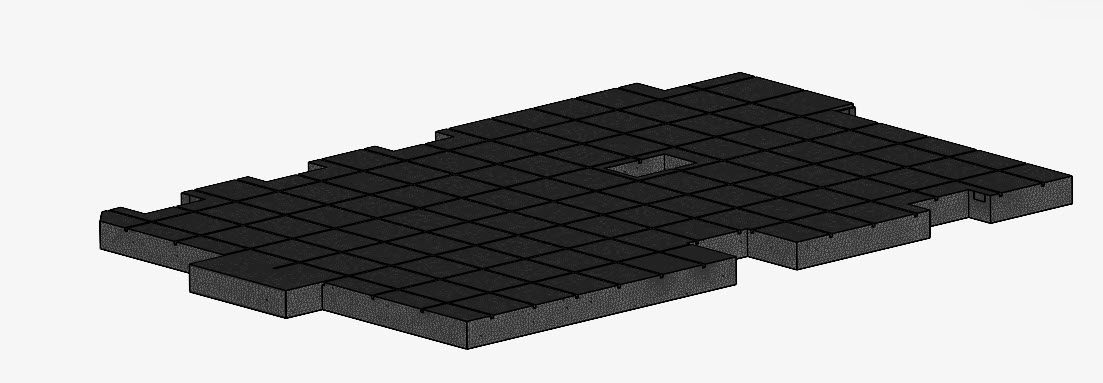
You do not need to use the Generate button to compute the mesh, as this action will be performed as part of the simulation run. Nonetheless, once the mesh is created, you can come back to this section and visualize it. It should look like follows:
Now the simulation setup is complete and you’re ready to start your analysis. For this, a simulation run needs to be created. A simulation run solves the physical model that we just defined.
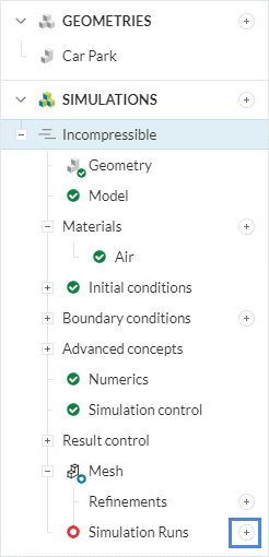
In order to create a new run, click the ‘+’ icon next to Simulation Runs.
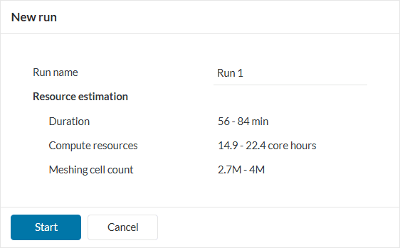
A dialog box will pop up asking you to name your run. Click the ‘Start’ button to launch the computation. When the process is finished, you will also be notified via e-mail.
After the simulation has finished, you will be able to analyze your results with the built-in post-processor.
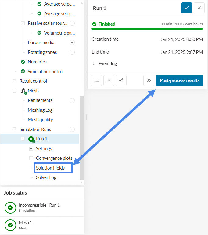
You can access the post-processor in two ways, by clicking on ‘Post-process results’ in the Run dialog or clicking on ‘Solution Fields’ under your simulation run. You will then be redirected to the post-processor. Before continuing, make sure that there are no predefined filters and that you are at the last timestep of the simulation.
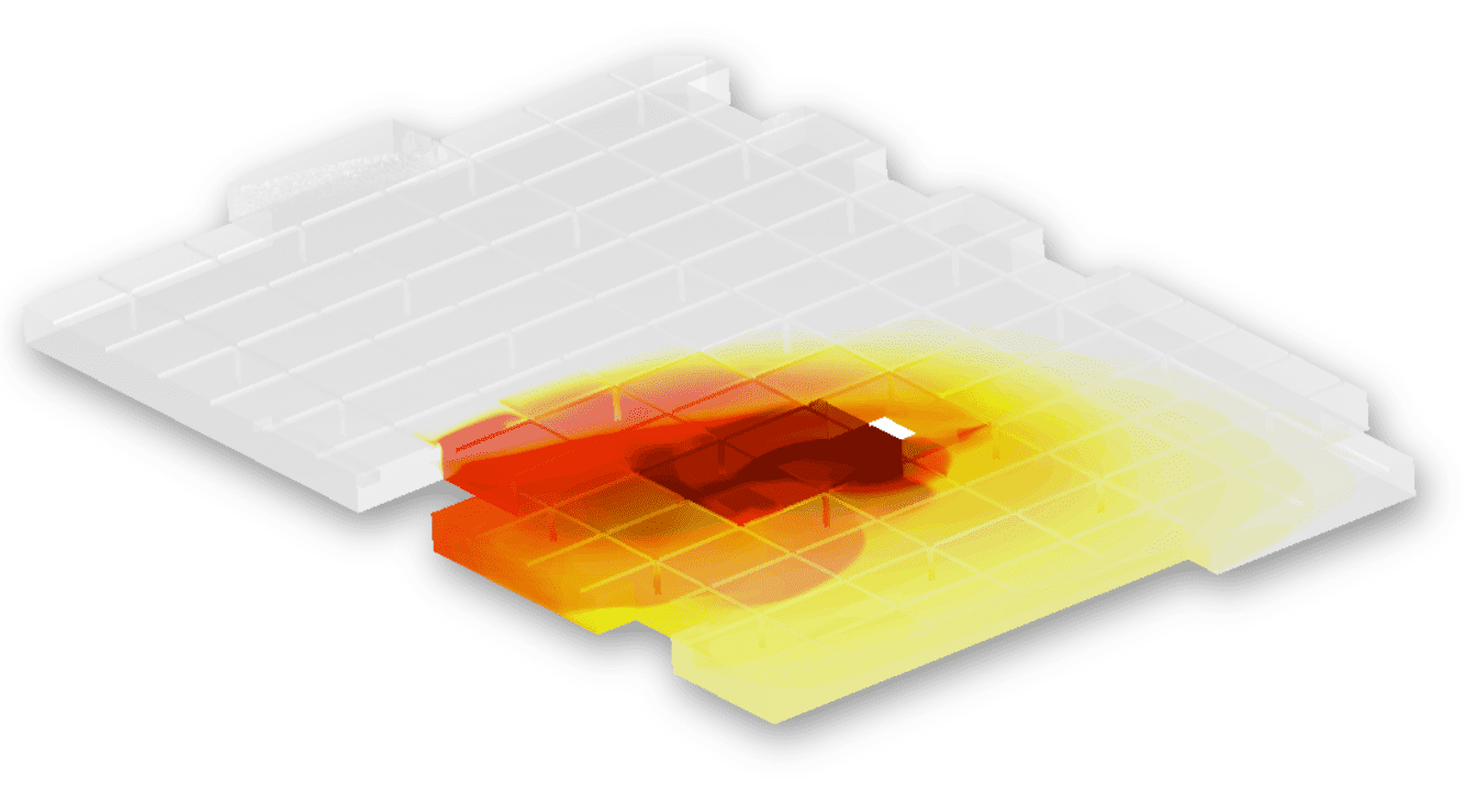
For this tutorial, we will visualize the areas where there is a high concentration of CO in the car park by using the Iso Volume filter. Iso volumes enable us to set a range for the output results from the simulation. Follow the steps below to find unsafe areas in the car park:
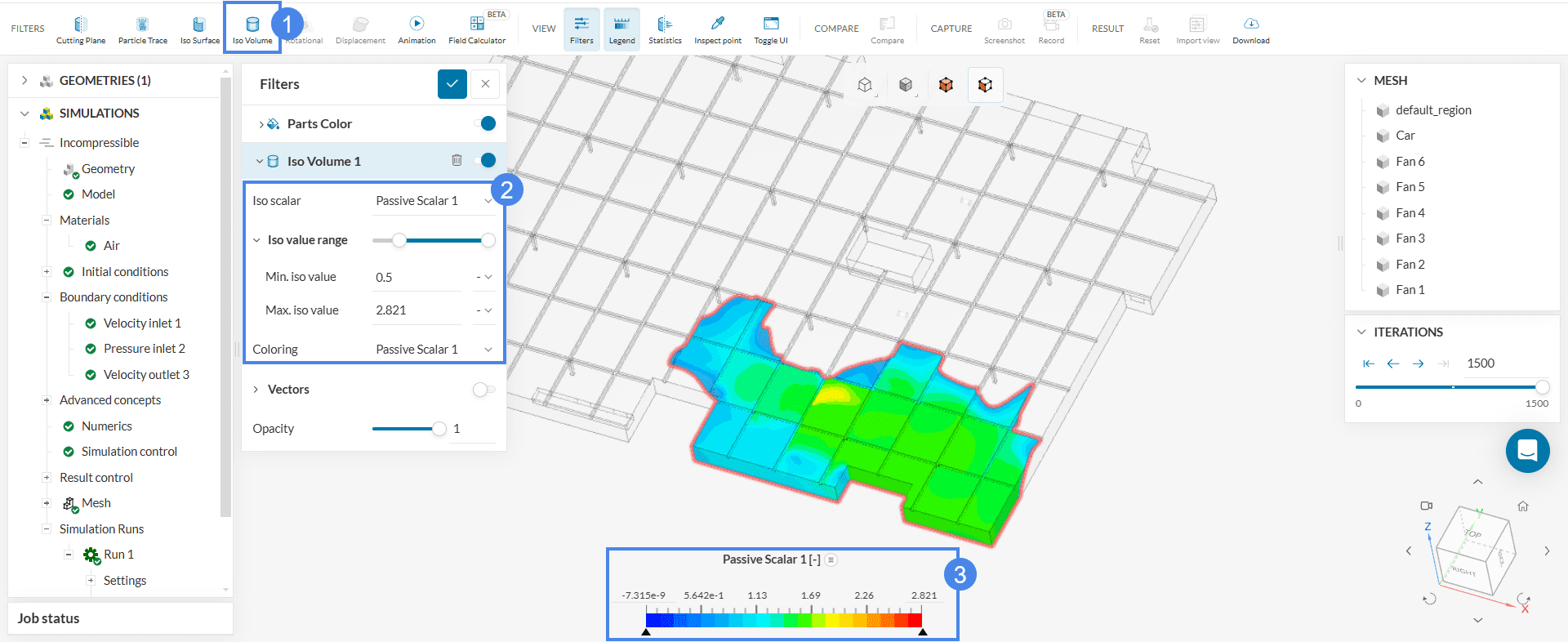
You can see from the figure above that the high concentration of CO only exists in the vicinities of the car.
To observe the concentration distribution of CO and the airflow across the parking, create a cutting plane as follows:
 .
.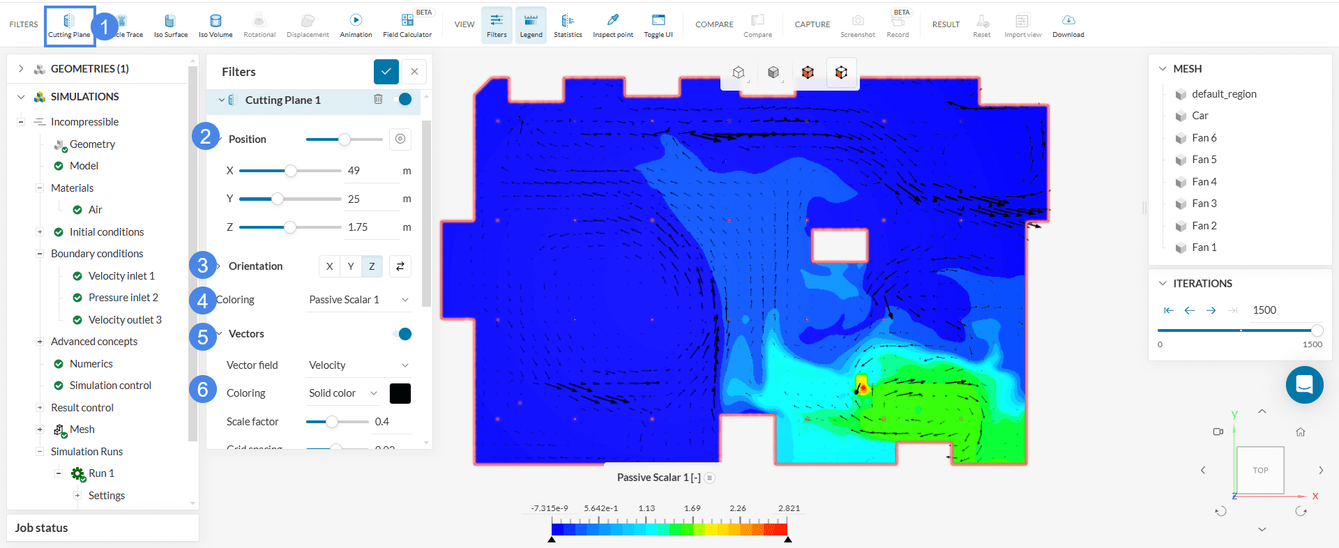
Based on the figure above, the airflow inside the car park with air jets is sufficient to decrease the concentration of CO inside the car park.
You can analyze the results further with the SimScale post-processor. Have a look at our post-processing guide to learn how to use it.
Congratulations! You finished the car park contamination tutorial!
Last updated: April 4th, 2026
We appreciate and value your feedback.
Sign up for SimScale
and start simulating now