Tutorial: Multiphase Flow Through a Globe Valve

This tutorial showcases how to use SimScale to run a transient, incompressible multiphase fluid simulation of water flowing through a globe valve.

Overview

This tutorial teaches how to:

• Set up and run a transient incompressible multiphase simulation using the Multi-purpose solver;
• Assign phase fractions as initial conditions;
• Assign boundary conditions, multiple materials, and other properties to the simulation;
• Mesh with the automatic meshing algorithm in Multi-purpose.

We are following the typical SimScale workflow:

1. Prepare the CAD model for the simulation;
2. Set up the simulation;
3. Create the mesh;
4. Run the simulation and analyze the results.

1. Prepare the CAD Model and Select the Analysis Type

To begin, click on the button below. It will copy the tutorial project containing the geometry into your Workbench.

The following picture demonstrates what is visible after importing the tutorial project.

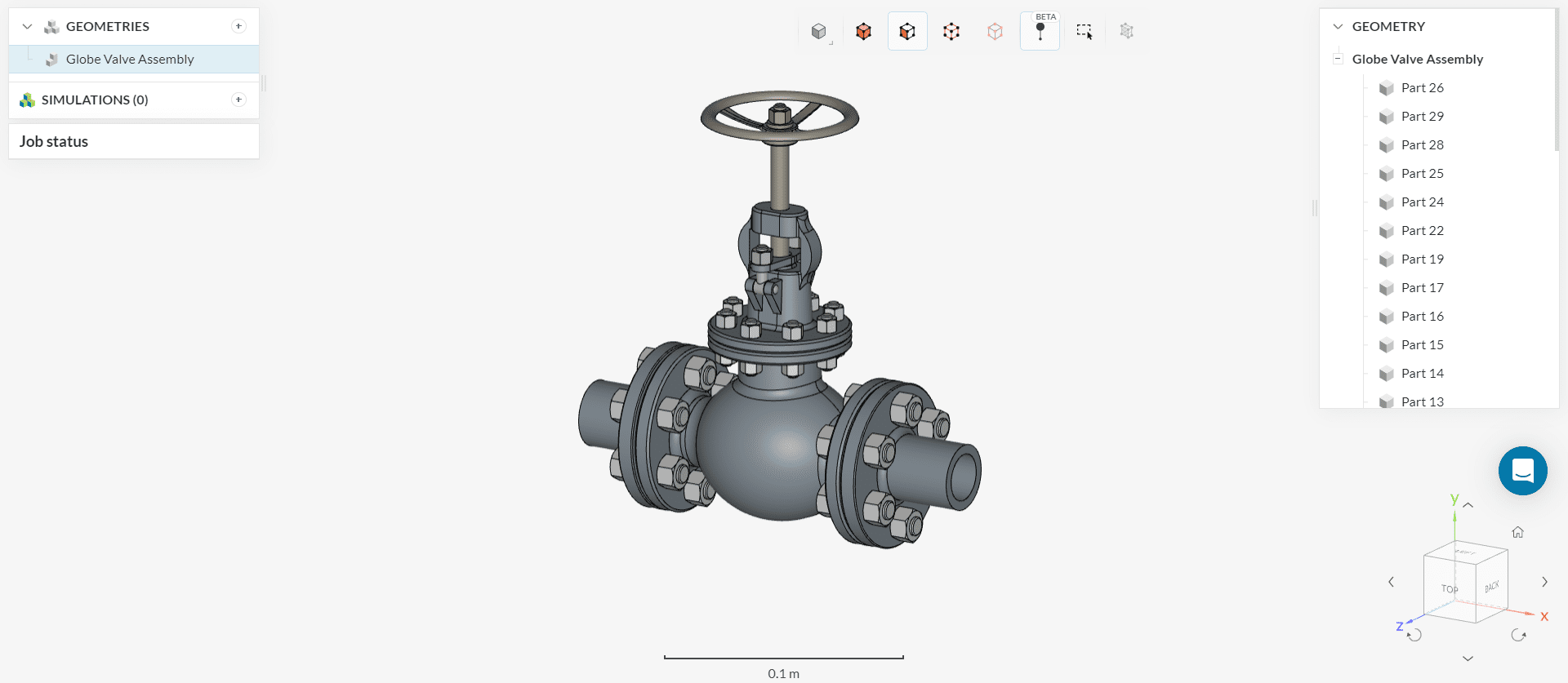
The geometry consists of the actual Globe Valve. It consists of multiple parts as can be observed in the scene tree.

1.1 Geometry Preparation

The geometry for this tutorial is not ready for CFD simulations. It contains multiple solid parts of the valve. For a multiphase analysis, we need a single flow volume region.

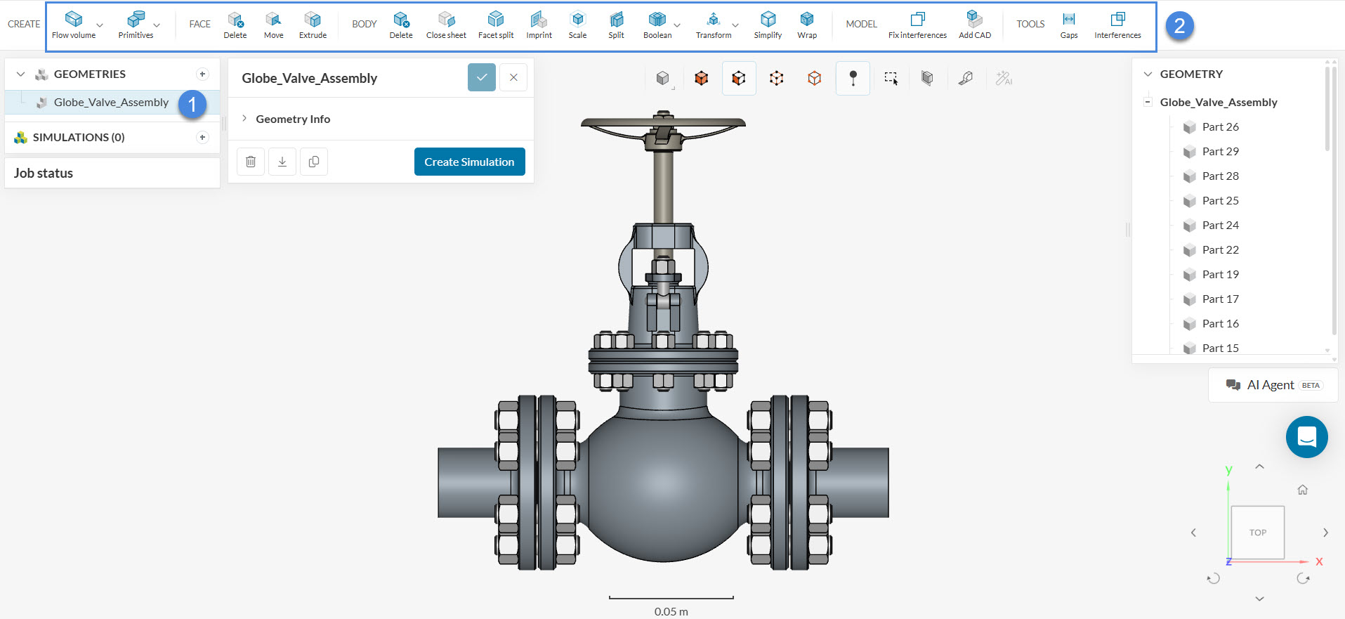
To create a flow volume click on the ‘Edit a Copy’ icon to enter the CAD edition mode.

Now perform the following steps:

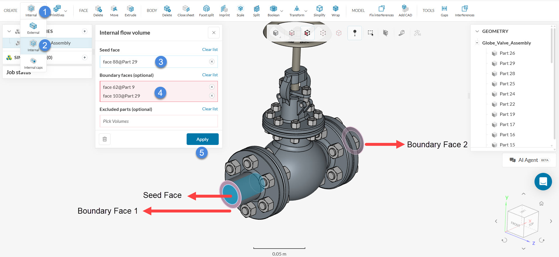
1. Select the ‘Internal Flow Volume operation’. This will lead to a settings panel where the user needs to define a seed face and boundary faces.
2. Assign the internal surface as a seed face.
3. Assign the two faces at the entry and exit boundaries as boundary faces.
4. Click ‘Apply’.

How To Create Flow Volume Extraction?

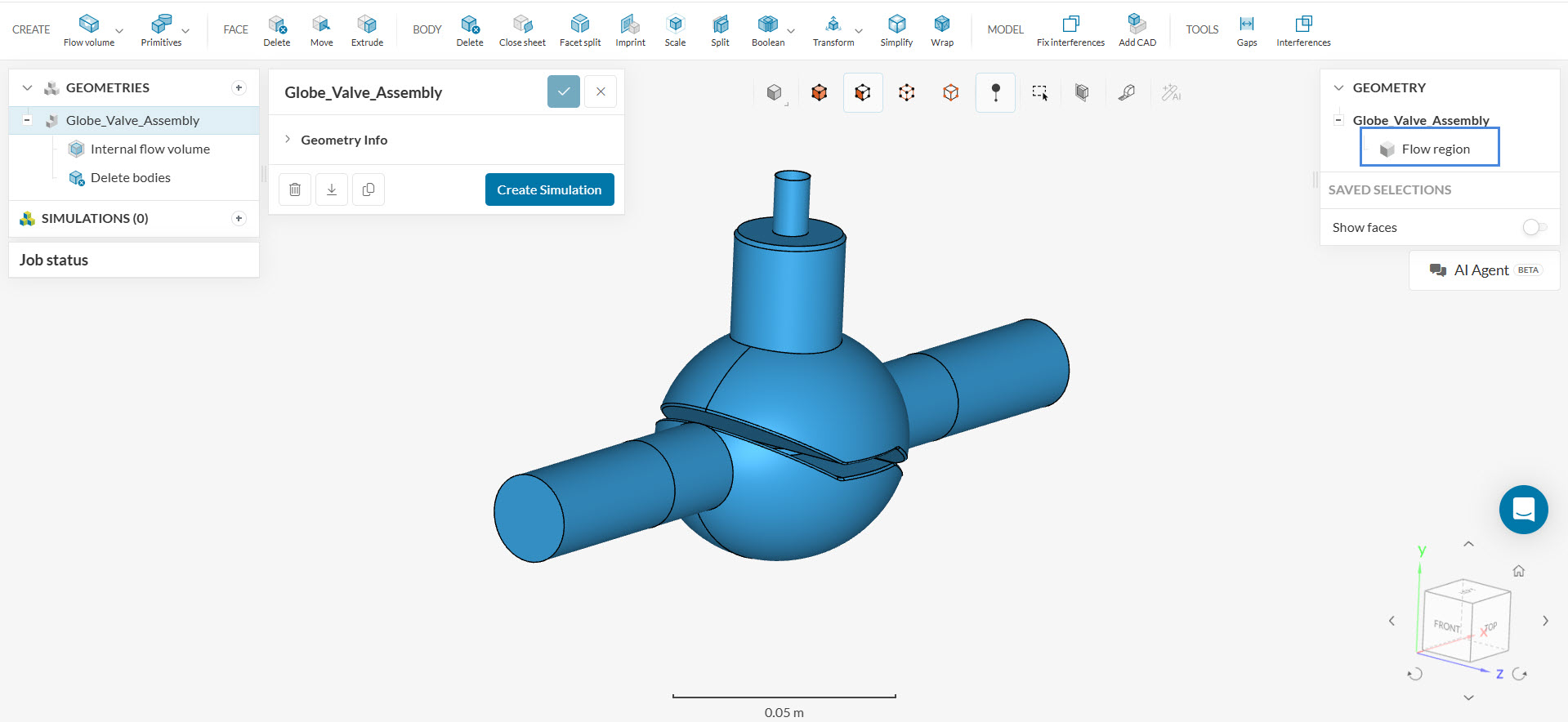
Notice that there is a new volume entity called Flow region under the parts list at the very end (see Figure 5). This is the only region that will involve the fluid interaction and which will be required for the CFD simulation.

To delete the remaining parts,

1. Select ‘Flow region’
2. Right-click to select ‘Invert selection’ from the drop-down
3. Choose the ‘Delete’ body option and select all bodies except the flow region, and hit ‘Apply’.

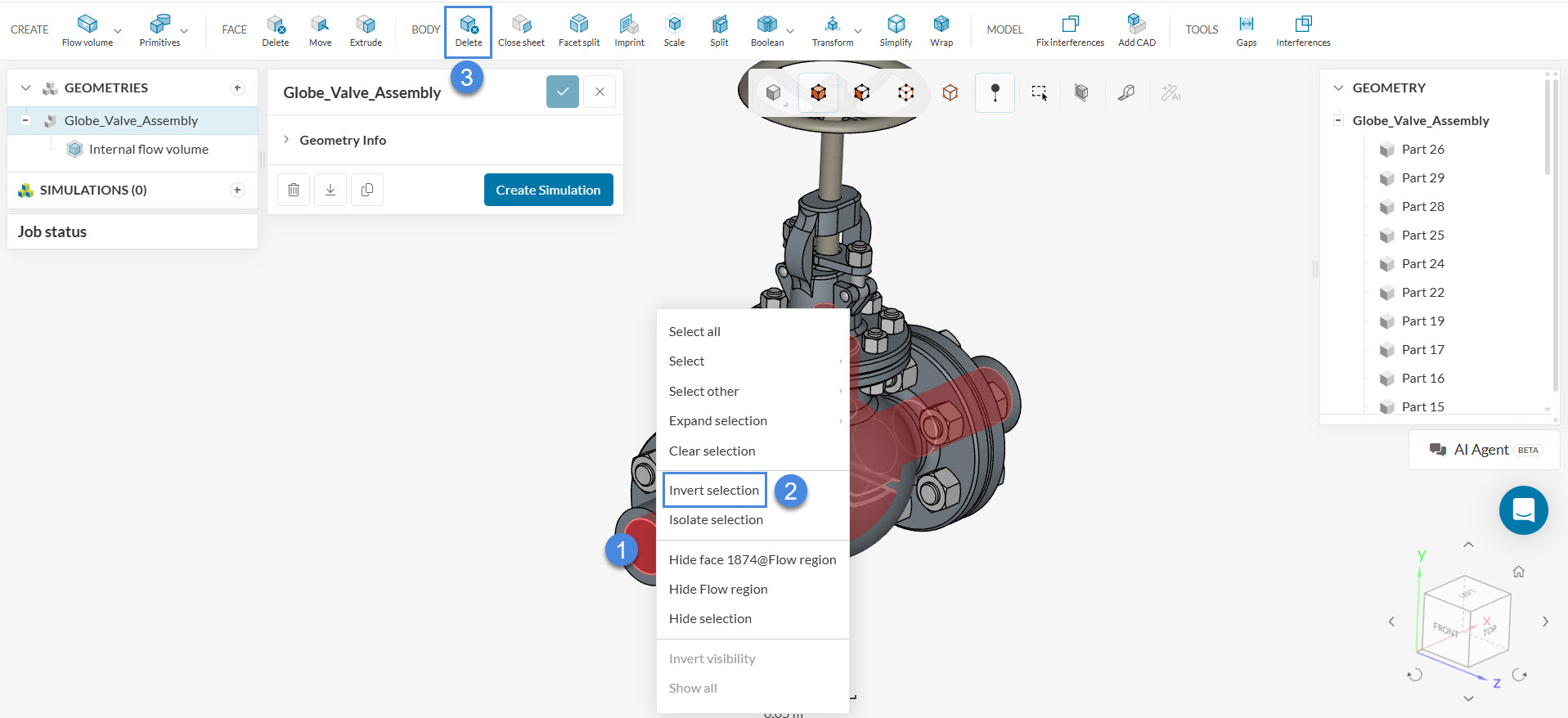
The user will be left with only the flow region. Use the ‘Save’ button to use this new geometry.

The modified geometry (Flow region) will appear under Geometries as a copy of the original valve geometry.

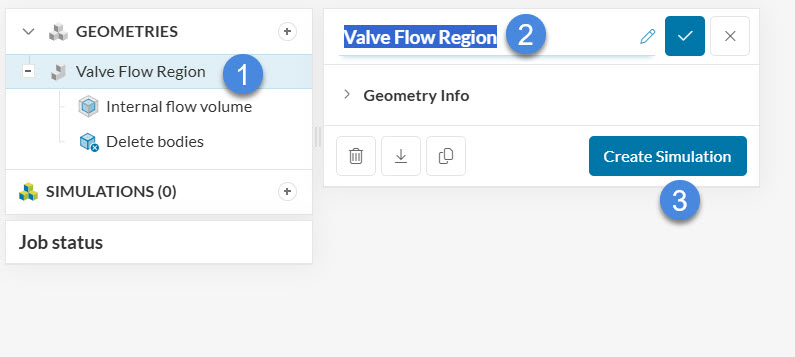
1.2 Create the Simulation

Rename the new geometry to ‘Valve flow region’ and hit the ‘Create Simulation’ button.

This will open the simulation type selection widget:

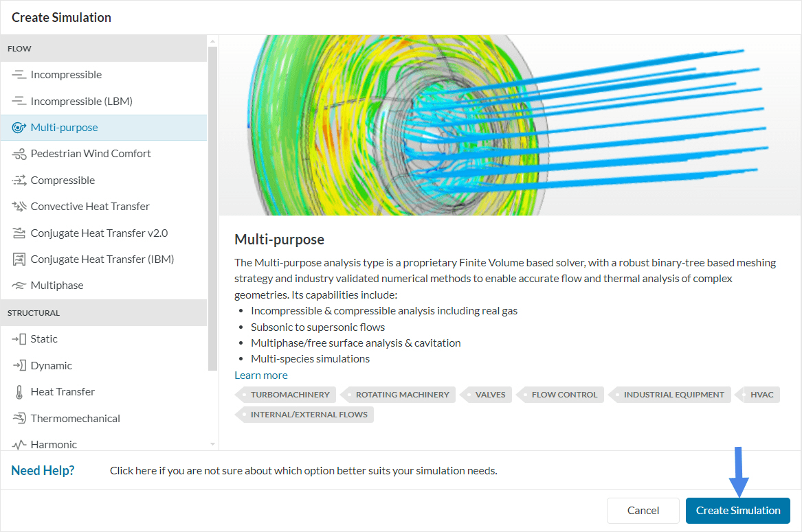
Choose ‘Multi-purpose’ as the analysis type and ‘Create Simulation’.

At this point, the simulation tree will be visible in the left-hand side panel. To run the simulation, it’s necessary to configure the simulation tree entries.

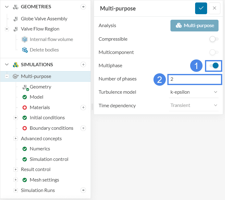
The global simulation settings will be adjusted for Time dependency to ‘Transient’ and the Toggle ‘Multiphase’ as in Figure 9. This is the only way a multiphase analysis can be performed.

We are simulating two materials, air and water. So let the number of phases be 2.

2. Pre-Processing: Setting up the Simulation

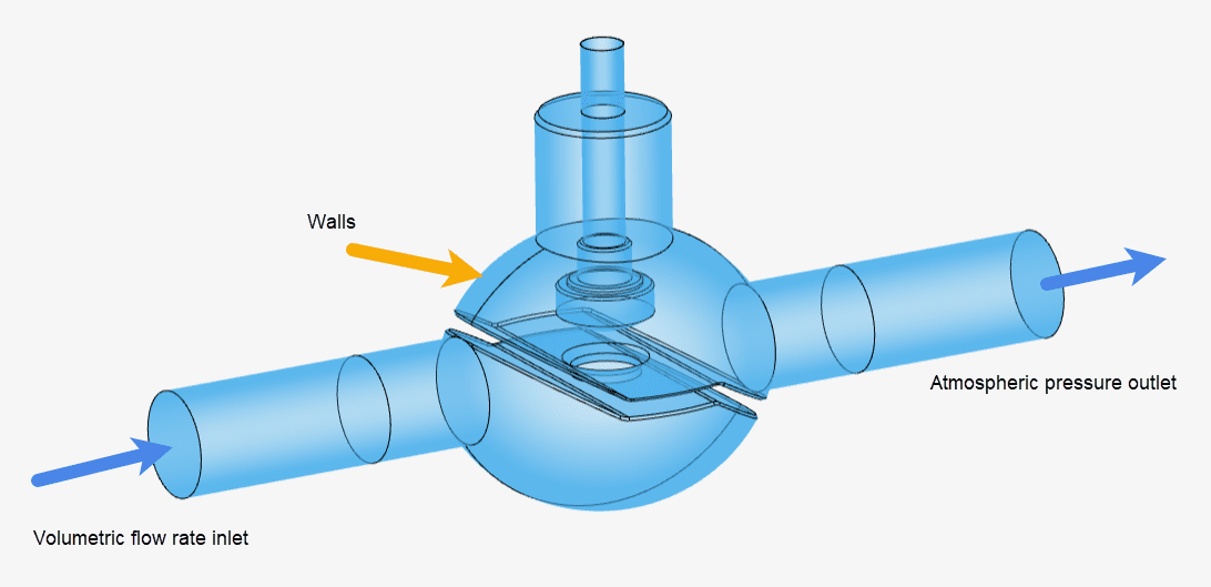
The following picture shows an overview of the boundary conditions.

2.1 Modeling Gravity

For the current scenario, we will include the gravitational acceleration effects in the flow physics as well.

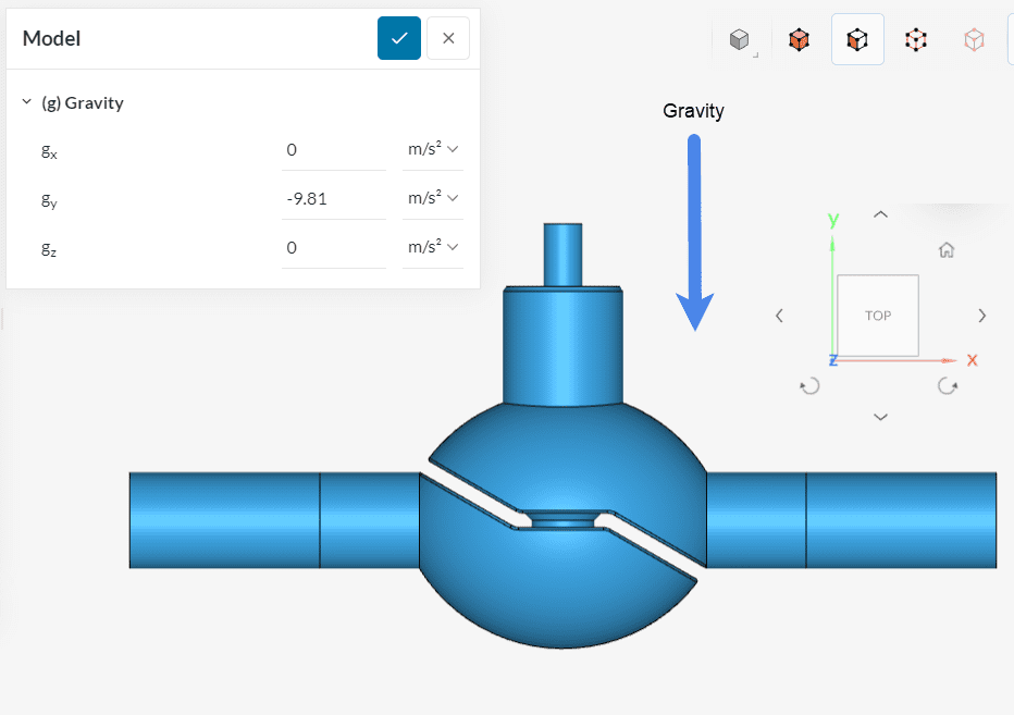
Click on ‘Model’ from the simulation tree and set g_y to ‘-9.81’ \(m/s^2\).

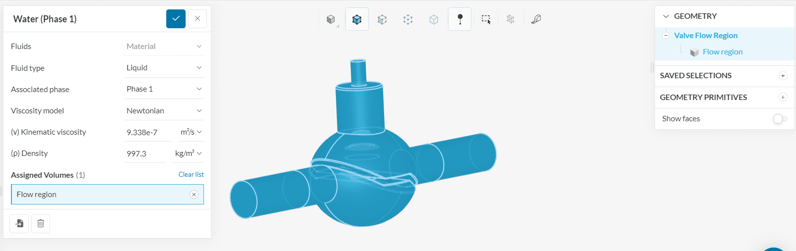
2.2 Define a Material

This simulation will begin with air initially present in the valve followed by water entering through the inlet. Therefore, this simulation will use air and water as two materials. Hence, click on the ‘+ button’ next to Materials. In doing so, the SimScale fluid material library opens, as shown in the figure below:

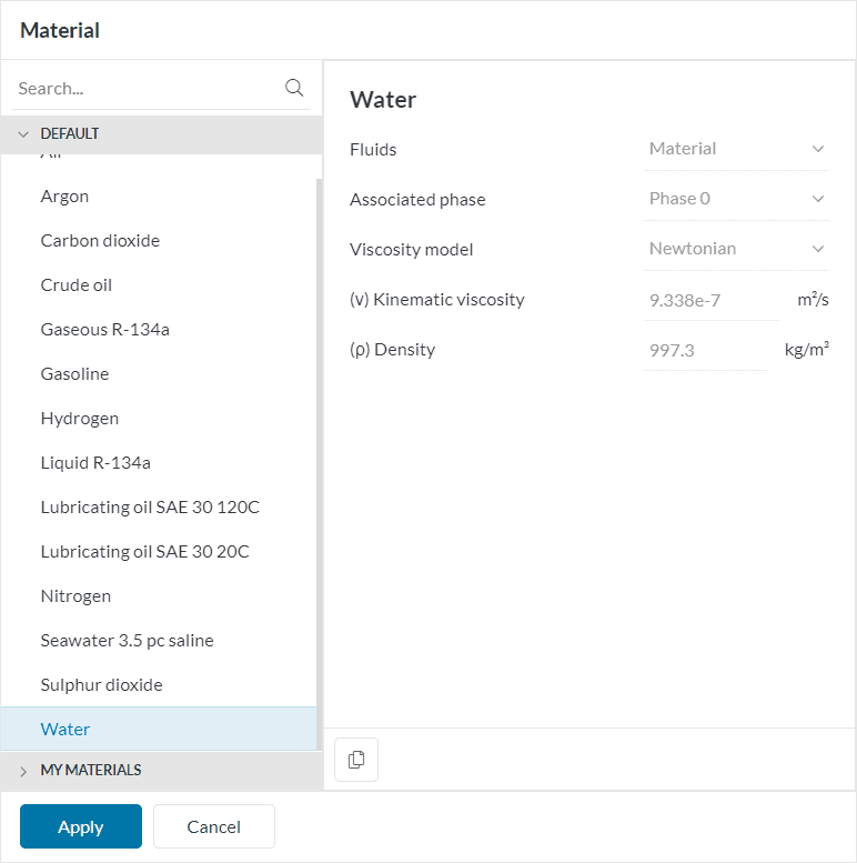
Select ‘Water’ and click ‘Apply’. Set the associated phase quantity to ‘Phase 1’. This means water will be recognized by a phase fraction value of 1 throughout the simulation. Keep the default values, and assign the entire Flow region to it (if not already by default).

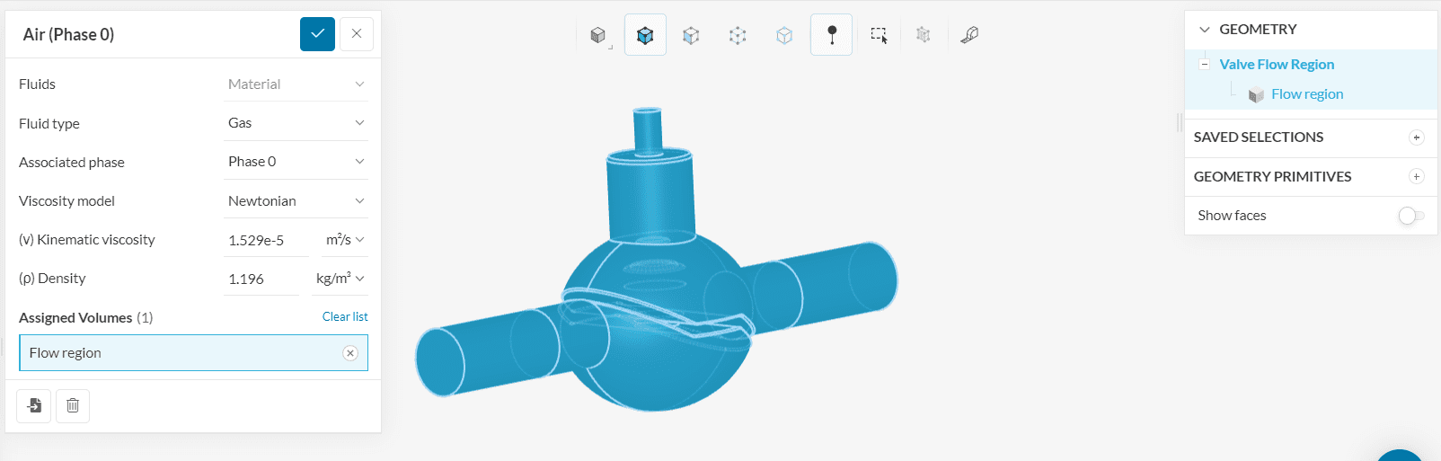
Repeat the same procedure for the material air. However, the Associated phase will be ‘Phase 0’.

2.2 Assign the Initial Conditions

As mentioned above, initially only air is present. This needs to be defined as an initial condition. Click on the ‘+’ icon next to Initial conditions > Phase fractions > Subdomains and perform the following:

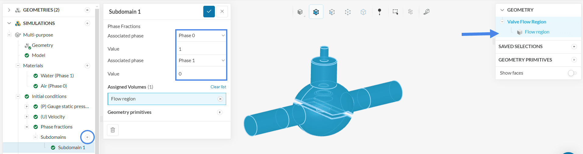
Ensure that the value of Phase 0 (air) is ‘1’ and Phase 1 (water) is ‘0’. Assign it to the entire flow region.

2.3 Assign the Boundary Conditions

In the next step, boundary conditions need to be assigned as shown in Figure 16. We have a velocity inlet and a pressure outlet. The rest are walls assigned by default.

a. Velocity Inlet

Click on the ‘+ button’ next to boundary conditions. A drop-down menu will appear, where one can choose between different boundary conditions.

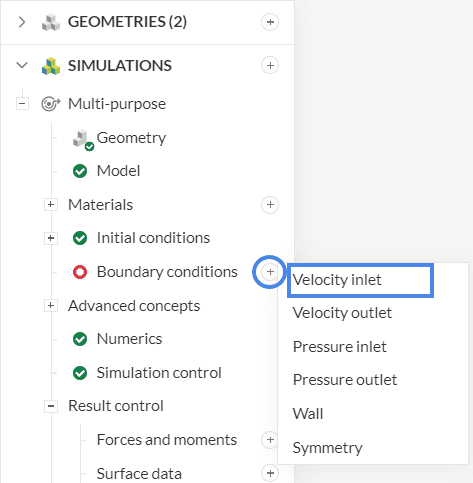
After selecting ‘Velocity inlet’, the user has to specify some parameters and assign faces. Please proceed as below:

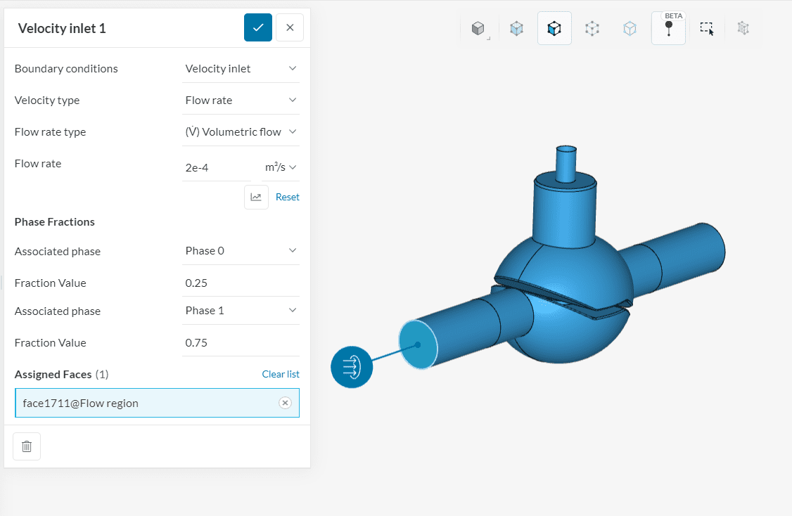
The Globe valve receives a mixture of 25% air and 75% water. This means the fraction value of phase 0 is 0.25 and that of phase 1 is 0.75. This mixture will enter through the inlet face at a volumetric flow rate of ‘2e-4’ \(m^3/s\).

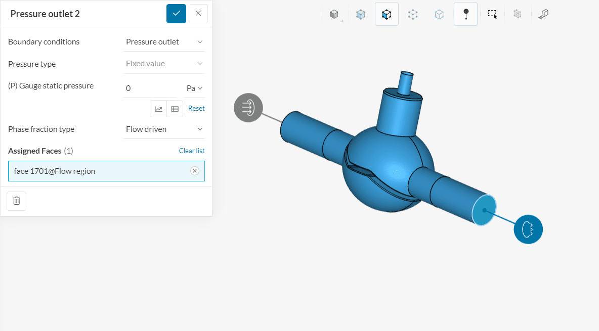
b. Pressure Outlet

Create a new boundary condition, this time a ‘Pressure outlet’, and select the outlet face. Make sure (P) Gauge Pressure is set to a fixed value of ‘0’ \(Pa\).

c. Walls

In Multi-purpose analysis, all the surfaces that act as walls are automatically treated likewise by the solver itself. So there is no need to assign them separately.

2.4 Simulation Control

Don’t worry about the numerical settings for this simulation, as their default values are optimized. Open the simulation control settings and change the following:

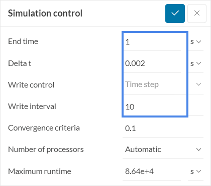
• End time:
  • The distance between the inlet and the outlet as well as the surface area at the inlet can be calculated using the Geometry Info. Using the flow rate and the inlet area an approximate value for the inlet velocity can be calculated too.
  • For at least 3 fluid passes (fluid entering and exiting the valve) the time can be calculated as ~0.8 seconds which can be rounded off to ‘1’ second. You can run it for longer end times until a desired convergence is obtained.
• Delta t: Keep it as ‘0.002’ seconds. The solver is robust to handle time steps over a large range of CFL number.
• Write interval: We will write results every ’10’ time steps.
• Maximum runtime: Transient simulations run longer. For this one set the maximum runtime to ‘8.64e4’ secs.

Keep the remaining settings as default. To know more about how to control the simulation read in detail here.

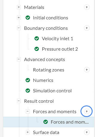
2.5 Result Control

Result control allows you to observe the convergence behavior globally as well as at specific locations in the model during the calculation process. Hence, it is an important indicator of the simulation quality and the reliability of the results.

a. Forces and Moments

For this simulation, please set a ‘Forces and moments’ control on the “plug” of the valve. Click on the ‘+’ icon under Result control> Forces and moments to open the settings panel as shown below:

Follow the steps carefully:

• Close the settings panel.
• Hide all the outer surfaces until the inner plug is visible.
  • To hide faces, select them and right-click to select the ‘Hide selection’ option from the drop-down. Continue until you see the plug as in Figure 21.

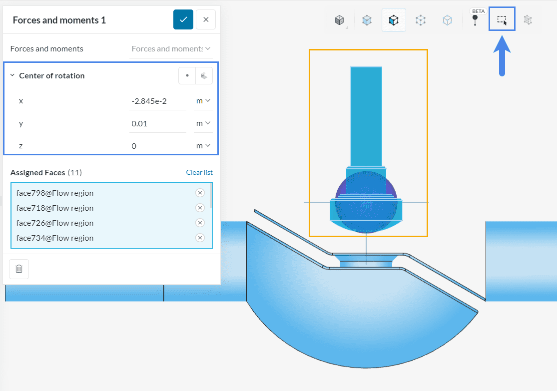
• Open the settings panel again by clicking on ‘Forces and moments 1’ (see Figure 20).
• Then activate the box selection tool and create a box from left to right to assign all 11 faces of the plug to this result control item.
• Enter the center of rotation coordinates.

c. Pressure Difference

We can also get the pressure difference between the inlet and the outlet directly as follows:

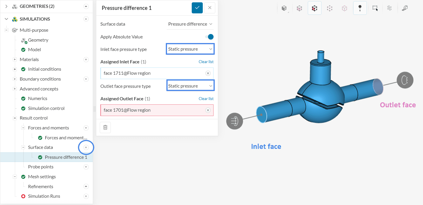
• Click on the ‘+’ icon next to Surface data.
• Set the inlet and outlet face pressure type to ‘Static pressure’.
• Assign the inlet and outlet faces as shown.
• Ensure that Apply Absolute Value is toggled on for a non-negative pressure difference.

3. Mesh

To create the mesh, we recommend using the Automatic mesh algorithm, which is a good choice in general as it is quite automated and delivers good results for most geometries.

In this tutorial, a mesh fineness level of 4 will be used. If you wish to undertake a mesh refinement study, you can increase the fineness of the mesh by sliding the mesh to higher refinement levels or using the region refinements.

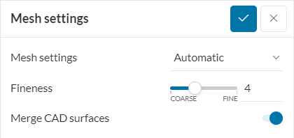
Since this is a transient simulation it is recommended to start with coarse mesh settings and gradually increase if required to save on core hours.

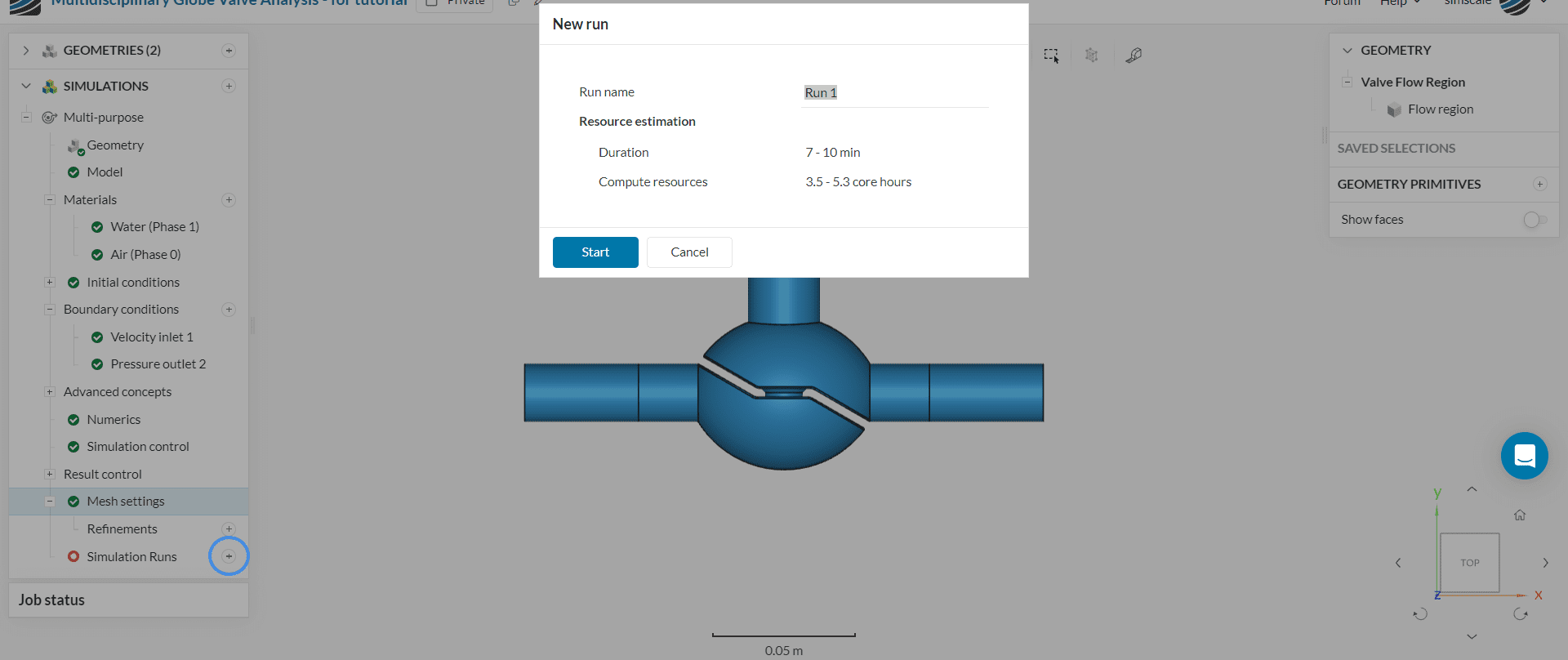
4. Start the Simulation

Now you can start the simulation. Click on the ‘+’ icon next to Simulation runs. This opens up a dialogue box where you can name your run and ‘Start’ the simulation.

While the results are being calculated you can already have a look at the intermediate results in the post-processor by clicking on ‘Solution Fields’ or ‘Post-process results’. They are being updated in real-time!

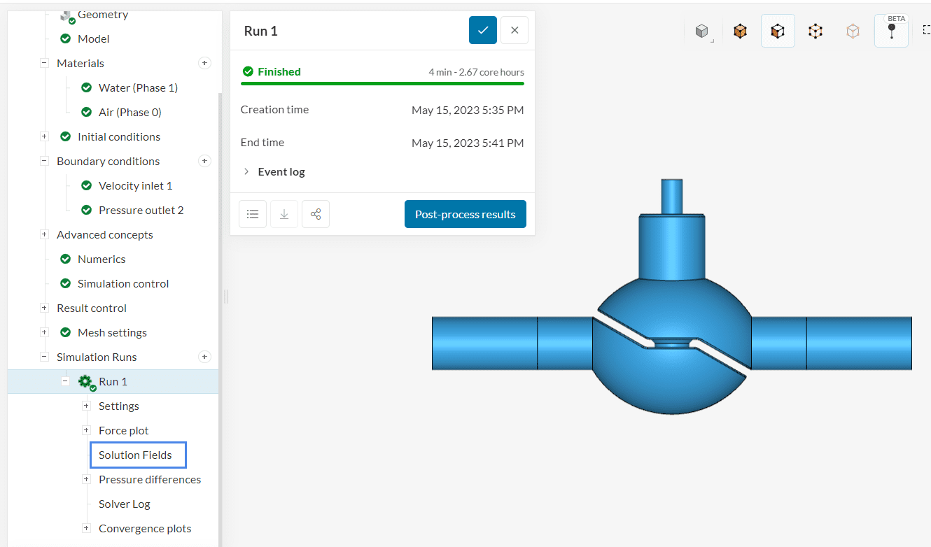
Depending on the instance chosen by the machine, it might take 5-10 minutes for the simulation to finish.

5. Post-Processing

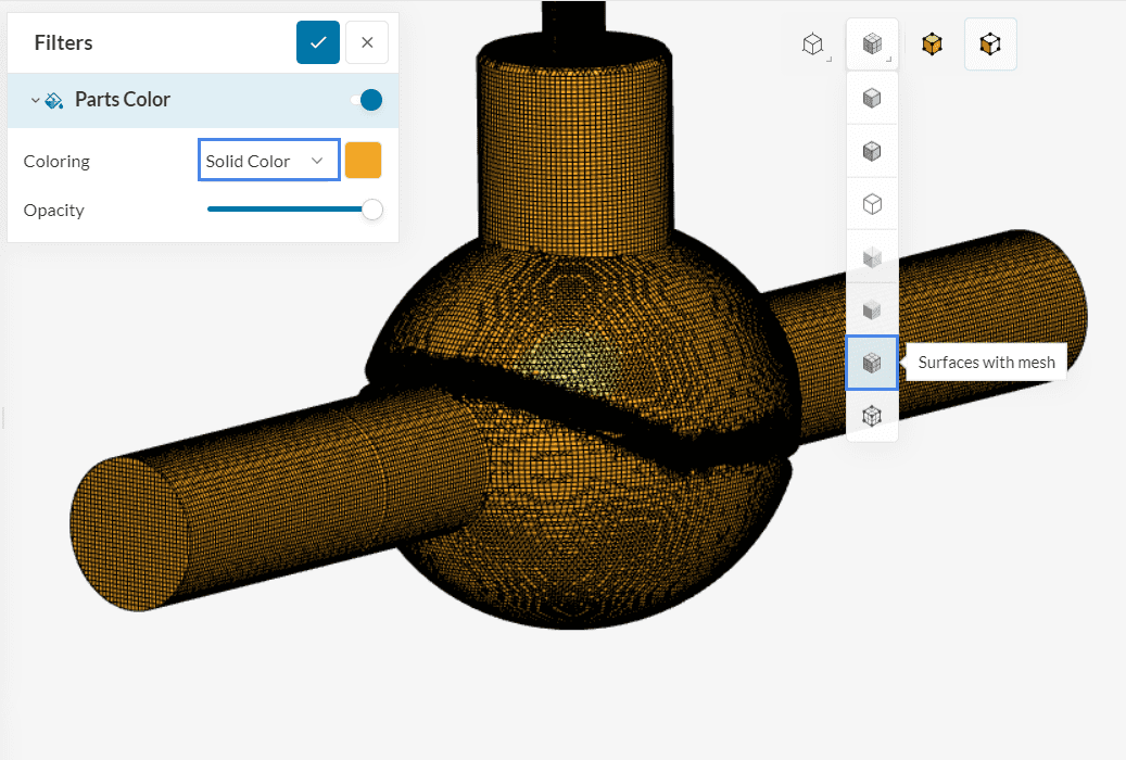
5.1 Visualizing the Mesh

Once inside the post-processor, under the Parts Color filter change Coloring to any solid color of choice and then change the render mode to Surfaces with mesh to show opaque surfaces of the CAD model with the mesh grid.

You can use the cutting plane filter to see the inside of the mesh generated:

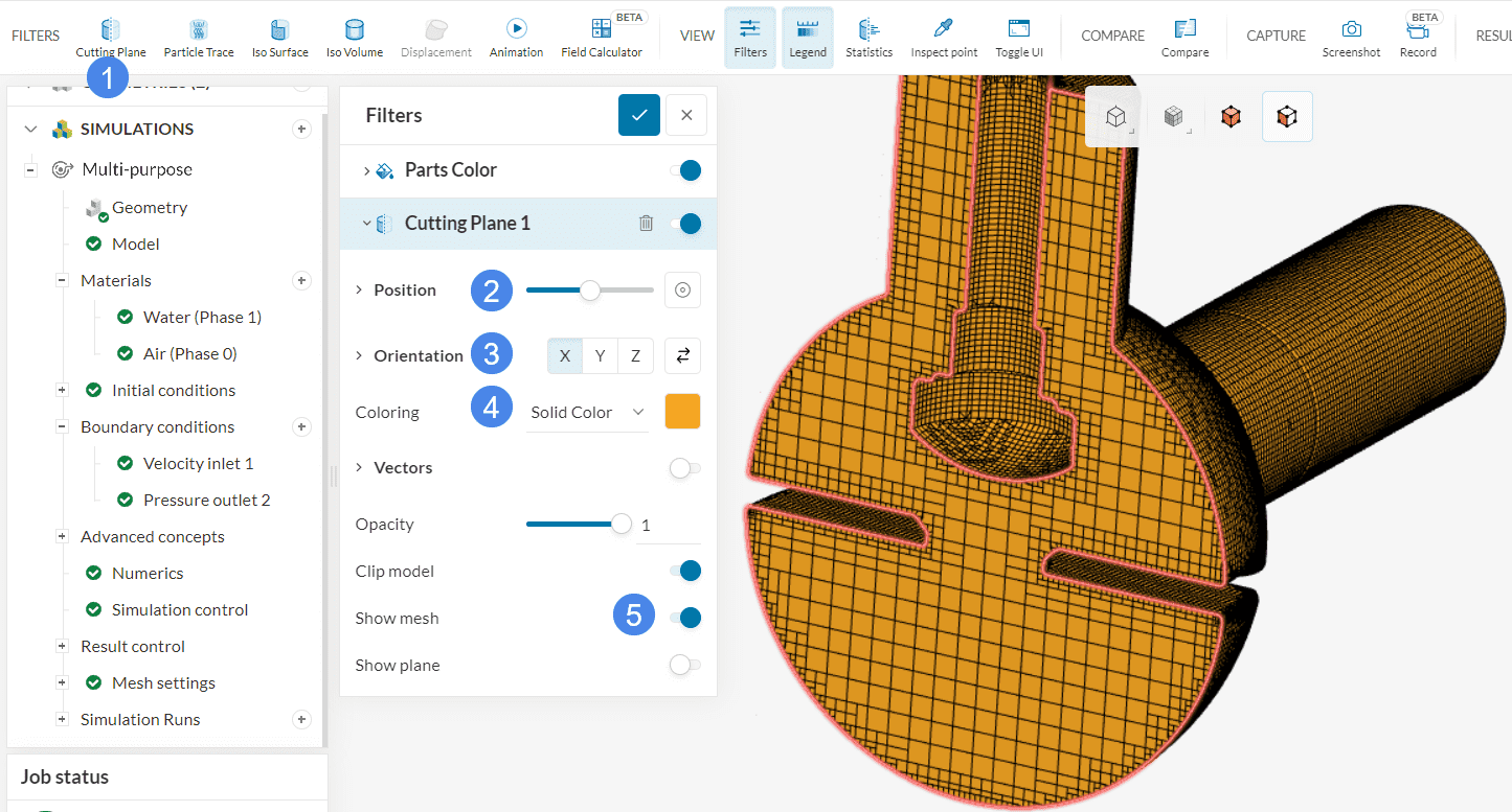
1. Hit the ‘Cutting Plane’ filter from the top ribbon.
2. Adjust the position accordingly.
3. Adjust the orientation to ‘X’ axis.
4. Change the Coloring to some contrasting solid color.
5. Toggle on Show mesh so that the mesh can be visible.

After a few seconds, you will see a clip showing the inside of your mesh. This mesh looks sufficient for this tutorial.

5.2 Forces and Moments on the Plug

The Forces and moments results are of particular interest in a simulation with a valve. The plug will be subjected to pressure forces from the incoming water. Hence, let’s inspect the resulting pressure forces and moments on the plug:

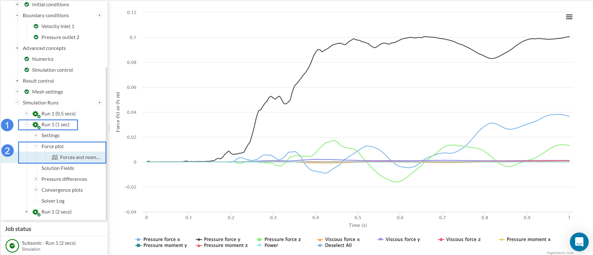
Figure 28 shows multiple runs performed with end times of 0.5, 1, and 2 seconds. For this tutorial purposes (end time of 1 second) the curves seem to be still fluctuating and more time steps might be required until a predictable pattern is observed.

5.3 Pressure Drop

One of the most important parameters to observe when evaluating the performance of a globe valve is how much the pressure drops after the water has flown through the valve.

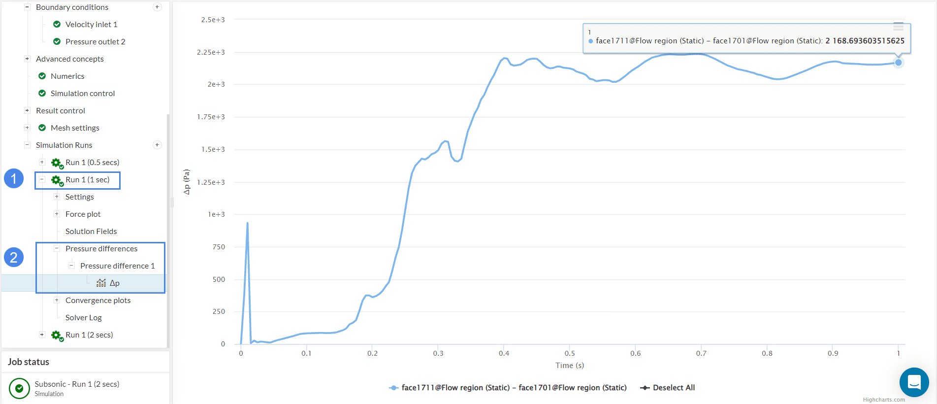
The transient nature of the pressure difference curve seems to be converging towards the end. Like the force plot, more time steps might be required to confirm a predictable pattern.

5.4 Particle Traces

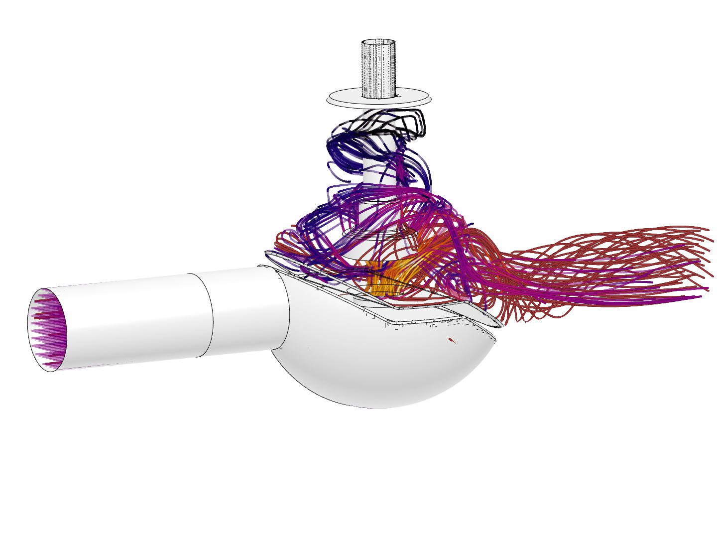
Streamlines can be a great tool to visualize flow patterns. Follow the steps below to show the flow streamlines inside the valve:

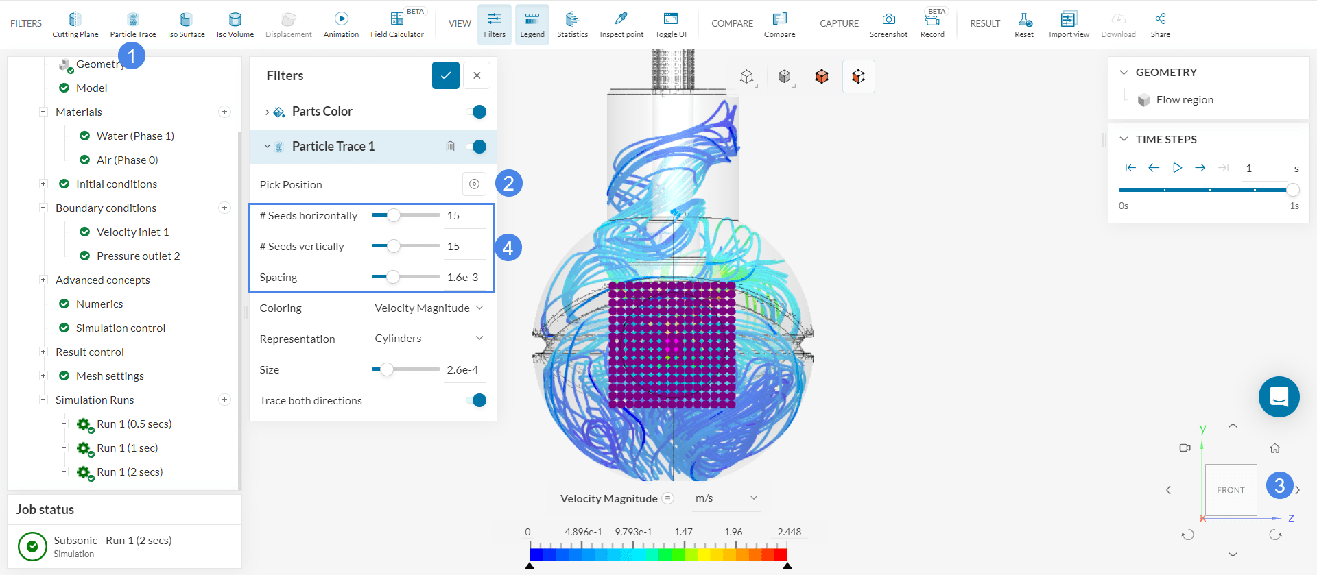
1. Remove any predefined filters and click on ‘Particle Trace’ on the top filters ribbon.
2. Ensure that the Pick position icon is activated.
3. Ensure that the front view for the geometry is aligned with the plane of your screen.
4. Choose the inlet as the seed face for the traces to be generated.

Now repeat the process, but this time select the outlet as a seed face.

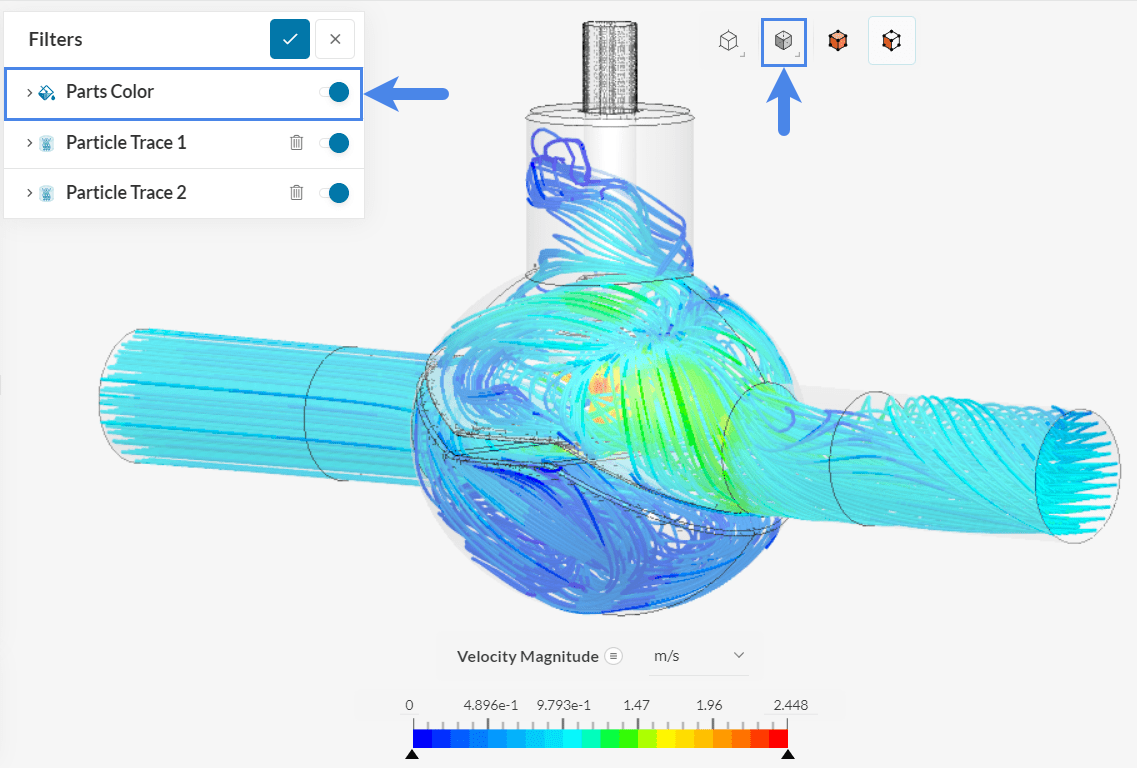
After the traces are created, you can adjust the render mode to ‘Translucent surfaces’ to give you a better view of the flow. Similarly, you can adjust the color of the parts for a better representation.

We can see that the flow follows a circular motion in the outlet region due to the rotatory motion of the turbine.

5.5 Pressure, Phase Fraction, and Velocity Vectors

Pressure

To get more details on the flow behavior inside the valve, use the Cutting plane filter.

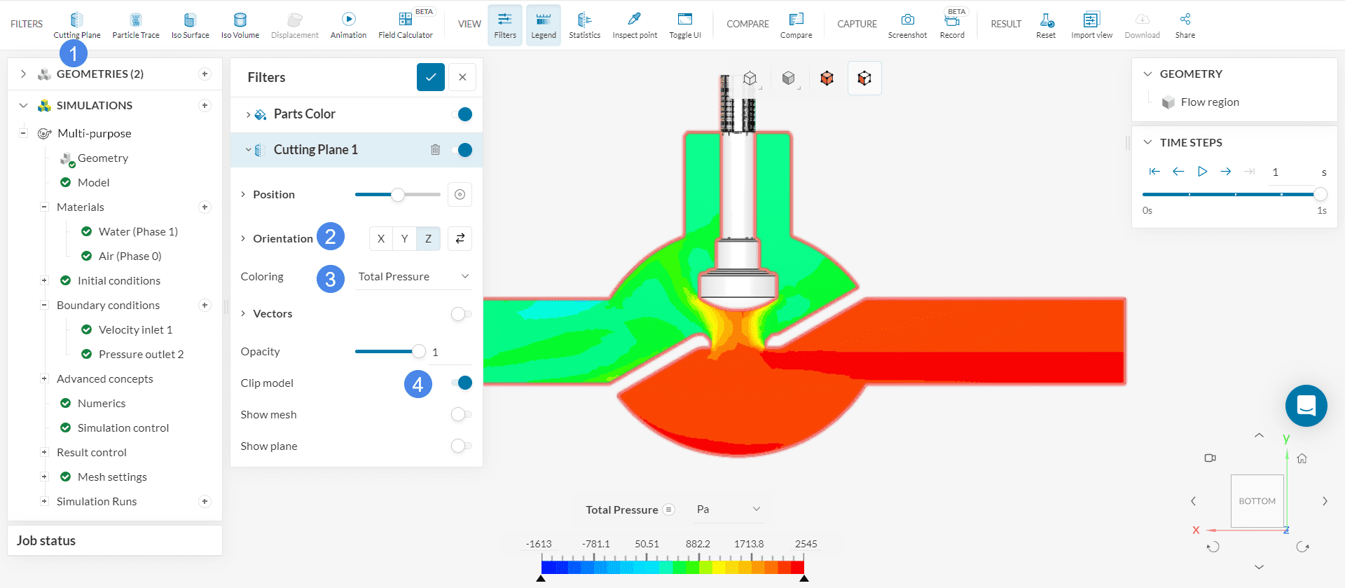
1. Create a ‘Cutting plane’ filter using the top ribbon.
2. Adjust the Orientation of the cutting plane to the ‘Z’ direction.
3. Set the Coloring of the plane to ‘Total Pressure’.

From Figure 32, you can see how the total pressure drops after the fluid air-water mixture crosses the valve plug section in the center and keeps decreasing towards the outlet.

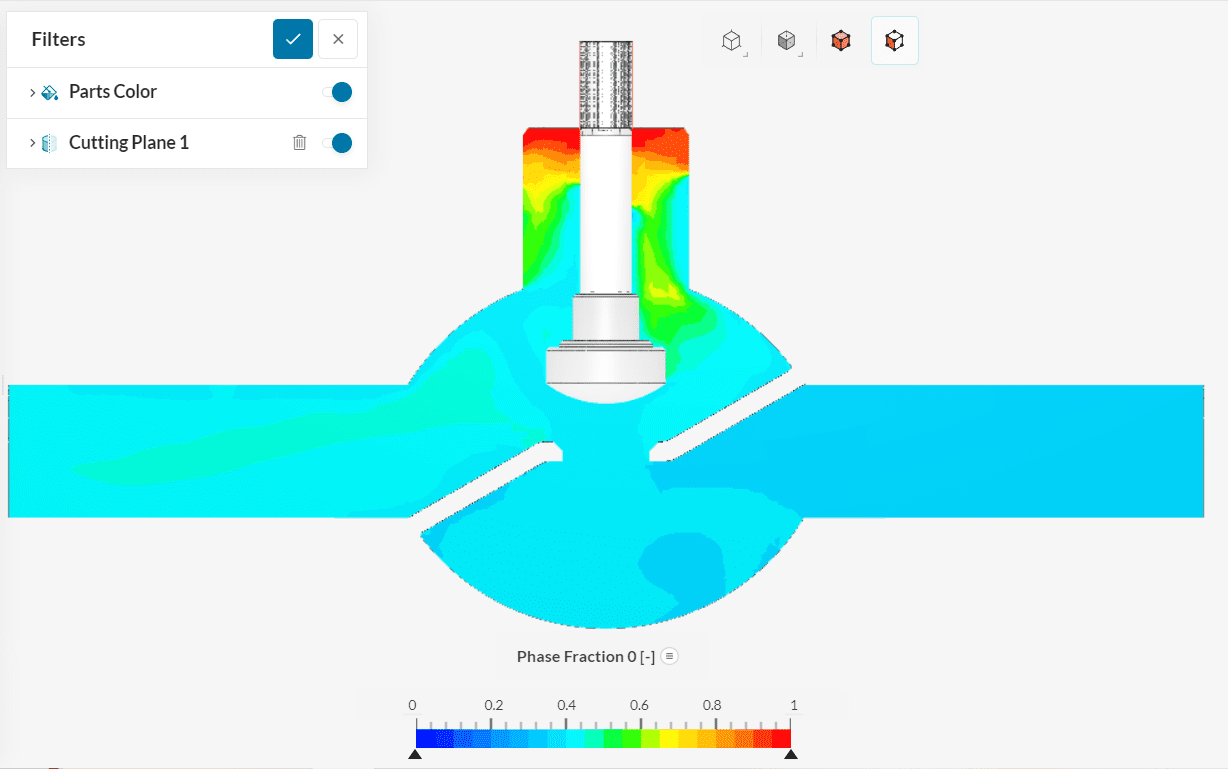
Phase Fraction

Different parameters can be viewed by changing the coloring. In Figure 33 air is visualized on the same cutting plane:

In Figure 34 water is visualized on the same cutting plane:

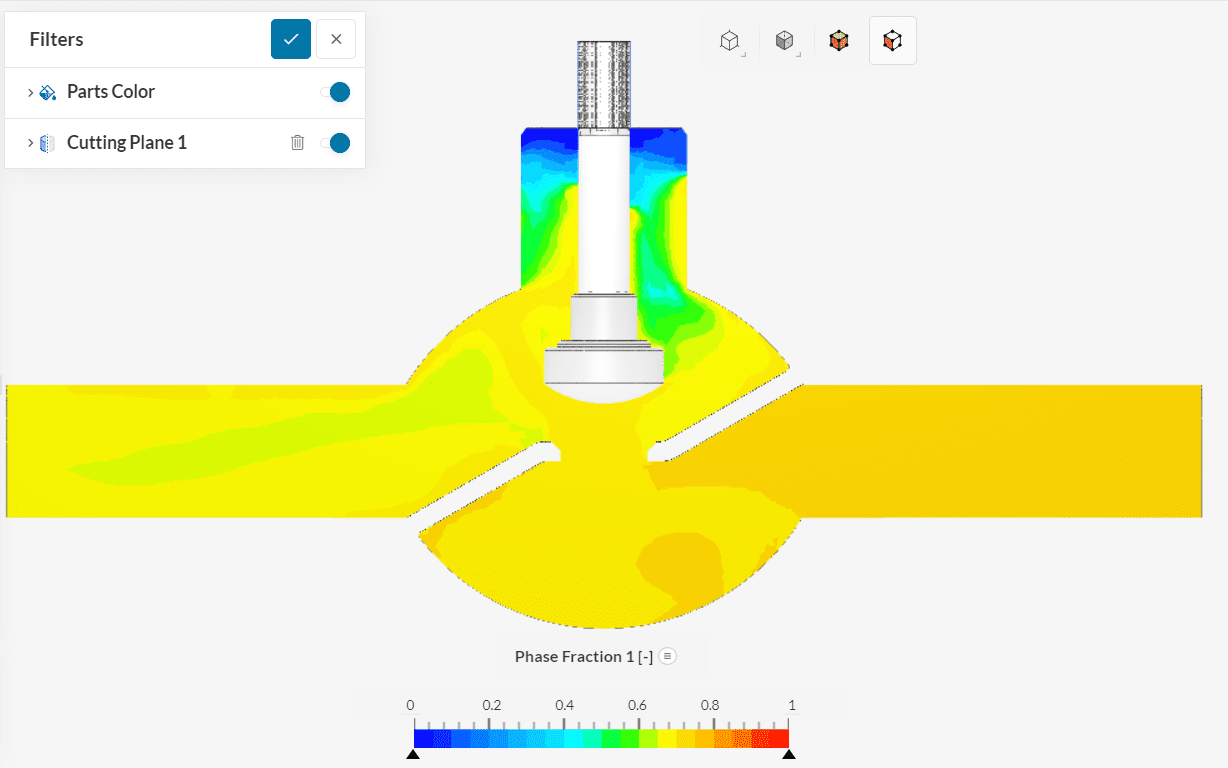
Figures 33 and 34 complement each other with their information. Most of the valve is filled with the air-water mixture with a water fraction between 0.6-0.8 and an air fraction between 0.2-0.4. The top part of the valve surrounding the plug has more air content.

Velocity Vectors

Vectors can also be interpreted on the cutting plane to understand the flow patterns.

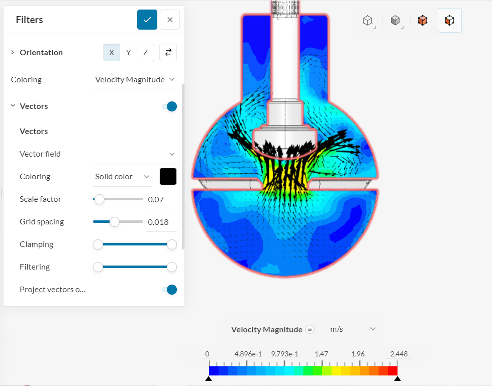
• Adjust the Orientation of the cutting plane to the ‘X’ direction.
• Change the Coloring of the plane to ‘Velocity Magnitude’.
• Toggle on Vectors and base its coloring with any contrasting solid color.
• Adjust the Scale factor of the vectors to ‘0.07’ and the Grid spacing to ‘0.018’.
• Enable the Project vectors onto plane option.

Longer vector lengths signify higher velocity magnitudes. The flow is not strong towards the bottom and top. Now change the orientation to the other two planes for more insights.

5.6 Animation

Any effect of the applied filters can be animated. Select ‘Animation’ from the top filter ribbon and click the play button under the Animation settings panel. Operate the animation commands as per your interests. Learn more.

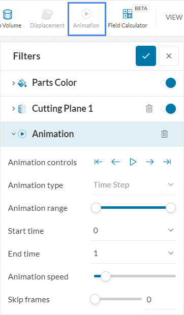
In this view, you can get insights into how the filling up of the globe valve takes place and what internal part designs are affecting the flow, allowing for optimizations in the design.

Analyze your results with the SimScale post-processor. Have a look at our post-processing guide to learn how to use the post-processor.

Last updated: October 22nd, 2024