Tutorial: Compressible Flow Simulation Around a Wing
This article provides a step-by-step tutorial for a compressible flow simulation around a wing.
Overview
This wing simulation tutorial teaches how to:
- Set up and run a compressible simulation
- Create and assign saved selections;
- Assign boundary conditions, material, and other properties to the simulation
- Mesh with the SimScale standard meshing algorithm;
- Visually assess the mesh quality
We are following the typical SimScale workflow:
- Prepare the CAD model for the simulation
- Set up the simulation
- Create the mesh
- Run the simulation and analyze the results
Attention!
This tutorial performs simulation with the Compressible analysis type which is only accessible to users with a Professional plan and those who are already on the Community plan. New Community users or those recently downgraded to the Community plan will no longer be able to perform this tutorial. See our pricing page to request additional features.
Learn with the video!
The following tutorial is also available in a video format with all steps described in equal detail. Experience this interactive way of learning and let us know your thoughts in the comments section.
1. Prepare the CAD Model and Select the Analysis Type
First of all, click the button below. It will copy the wing simulation tutorial project containing the geometry into your workbench.
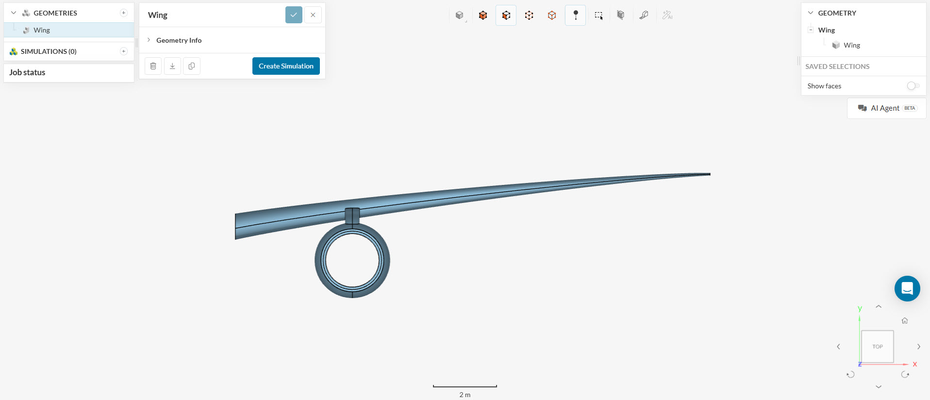
The following picture demonstrates what should be visible after importing the tutorial project:
1.1 Creating the Flow Region
To run a wing simulation where you can visualize the airflow, the first step is to create a flow region. This page gives you an overview of SimScale’s flow volume extraction operations.
For this project, the air domain will be created with an External Flow Volume operation, which is available in SimScale’s workbench after clicking on the imported geometry. To modify a CAD model, simply select the geometry from the list—the available CAD operations will then appear in the top toolbar. You can either work directly on the original model or create a duplicate and apply your changes to the copy.
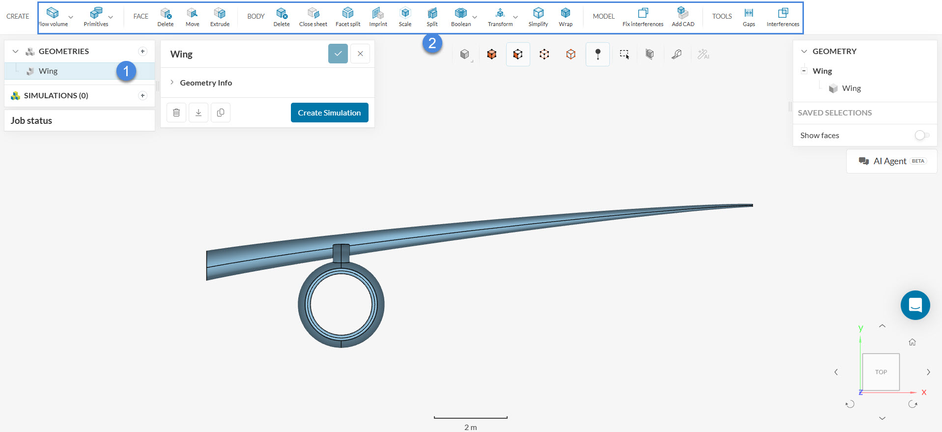
- Select the ‘Wing’ geometry from the GEOMETRIES panel
- The CAD operations should appear on top
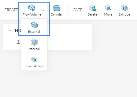
This will allow you modify your model, and you’ll be able to perform several CAD operations within the same user interface. Once the geometry is selected, you will find a large number of available operations, which are accessible from the top bar. Using Figure 4 as a reference, you can hover over the ‘Create – Flow Volume’ icon to reveal the drop-down menu, and select the ‘External’ option:
At this point, you are prompted to define the extent of the flow volume region. Please proceed as shown below:

- After creating the external flow volume operation, please define the minimum and maximum coordinates (in meters) as follows:
Minimum x: ‘0’
Maximum x: ’60’
Minimum y: ‘-90’
Maximum y: ’90’
Minimum z: ‘-120′
Maximum z: ’60’ - Hit ‘Apply’ when the coordinates are set.
Now the geometry is almost ready to start setting up the simulation. Before doing so, we need to delete the volume that represents the solid wing. To do that, please create a Delete body operation and proceed as below:
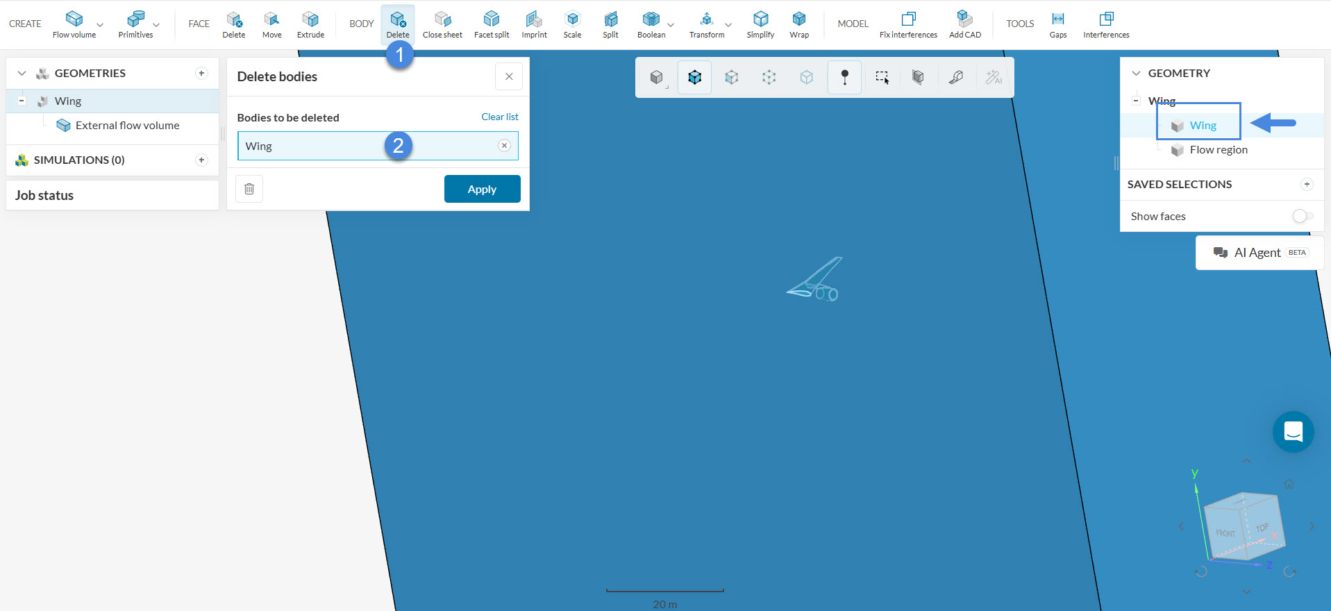
- Create a ‘Body – Delete’ operation from the top bar.
- Select the ‘Wing’ volume from the GEOMETRY panel.
- Hit ‘Apply’ to run the operation.
- Once done, the geometry will be ready.
Did you know?
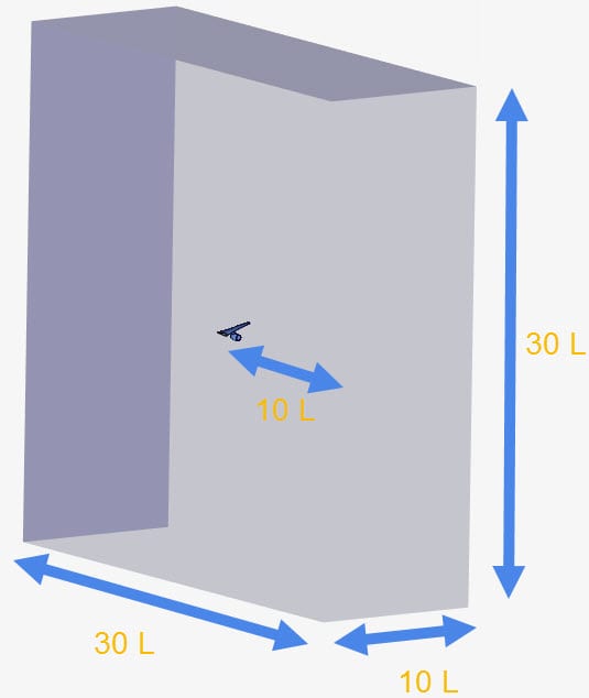
The boundaries of the domain should be far away from the wing. This is necessary to ensure that the flow near the wing won’t be affected by the conditions at the boundaries.
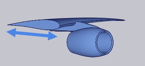
In a wing, chord length is the distance between the leading and trailing edges.
In general, the bigger the enclosure, the better. However, keep in mind that a big enclosure will increase the mesh cell count. Find below the minimum recommended size for the enclosure, in terms of chord lengths (L):
1.2 Create the Simulation
The modified version of the CAD model is overwritten under the Geometries list wit same name. You can select this volume and change its name if you would like. At this point, we are ready to create a simulation for the new geometry:
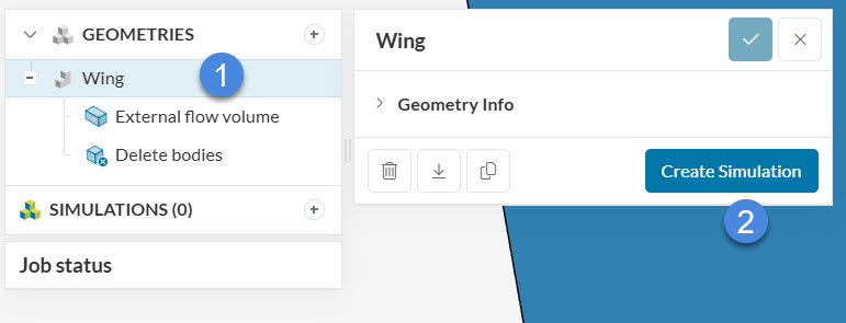
Hitting the ‘Create Simulation’ button leads to the following options:
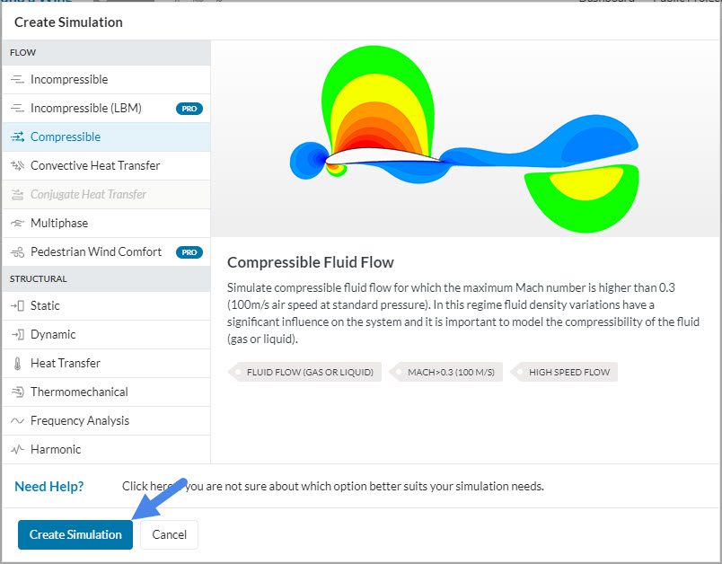
Choose ‘Compressible’ for analysis type and hit ‘Create Simulation’.
Now the global simulation setups pop up:
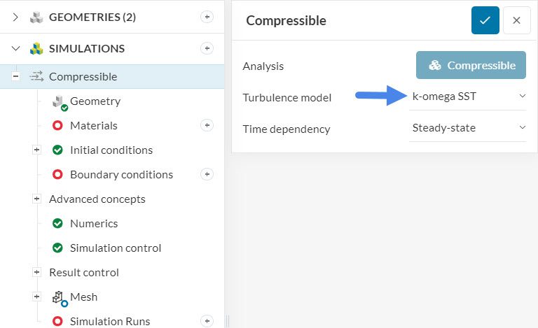
Set the turbulence model to ‘k-omega SST’.
2. Assigning the Material and Boundary Conditions
2.1 Define a Material
This simulation will use air as fluid material. Therefore click on the ‘+ button’ next to Materials. Doing this opens the SimScale fluid material library as shown in the figure below:
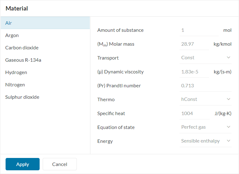
Select ‘Air’ and click ‘Apply’. Afterward, a tab with properties opens up. You can leave the default values and assign them to the entire flow region.
2.2 Assign the Boundary Conditions
To have an overview, the following picture shows the boundary conditions applied for this simulation:
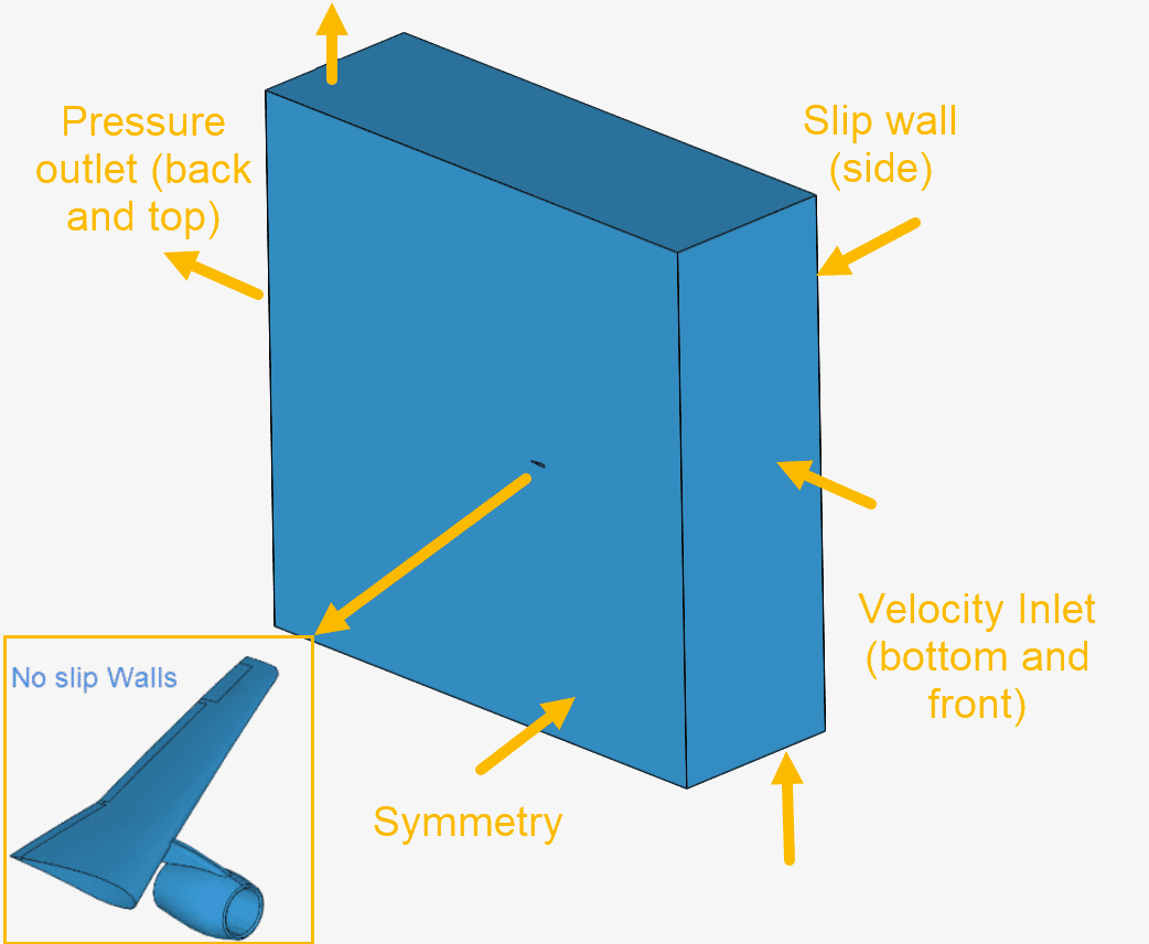
Using Figure 13 as a reference, the boundary conditions will be assigned.
a. Walls – Slip
Follow the instructions presented in the picture below to add a new boundary condition:

- After hitting the ‘+ button’ next to boundary conditions, a drop-down menu will appear, where one can choose between different boundary conditions.
- Select a ‘Wall’ boundary condition.
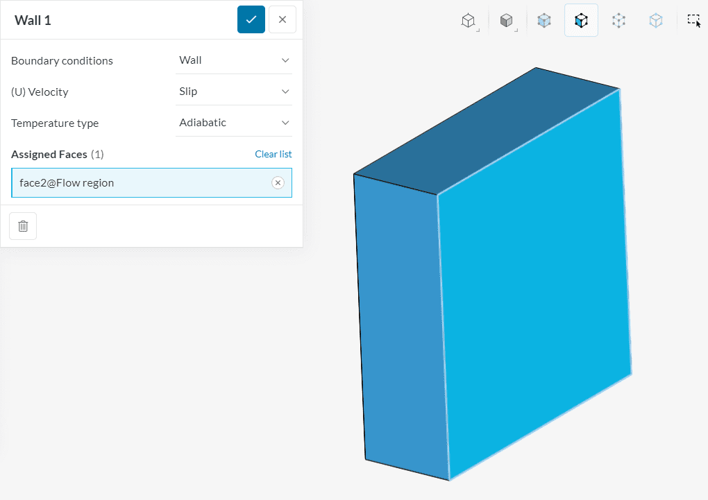
Change (U) Velocity to ‘Slip’ and Temperature type to ‘Adiabatic’. Assign the side enclosure boundary to it.
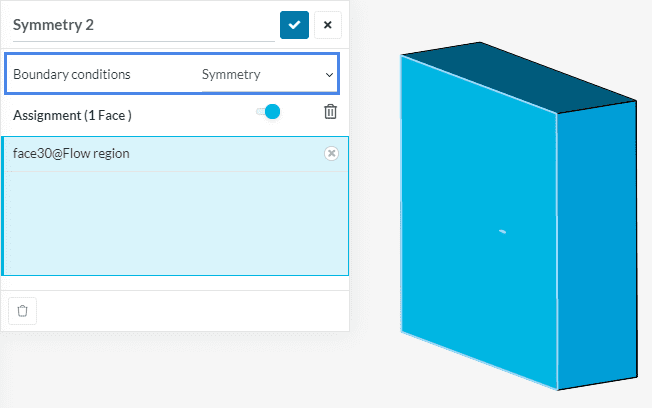
b. Symmetry
Create a new boundary condition, but this time choose ‘Symmetry’. Assign it to the enclosure face adjacent to the wing.
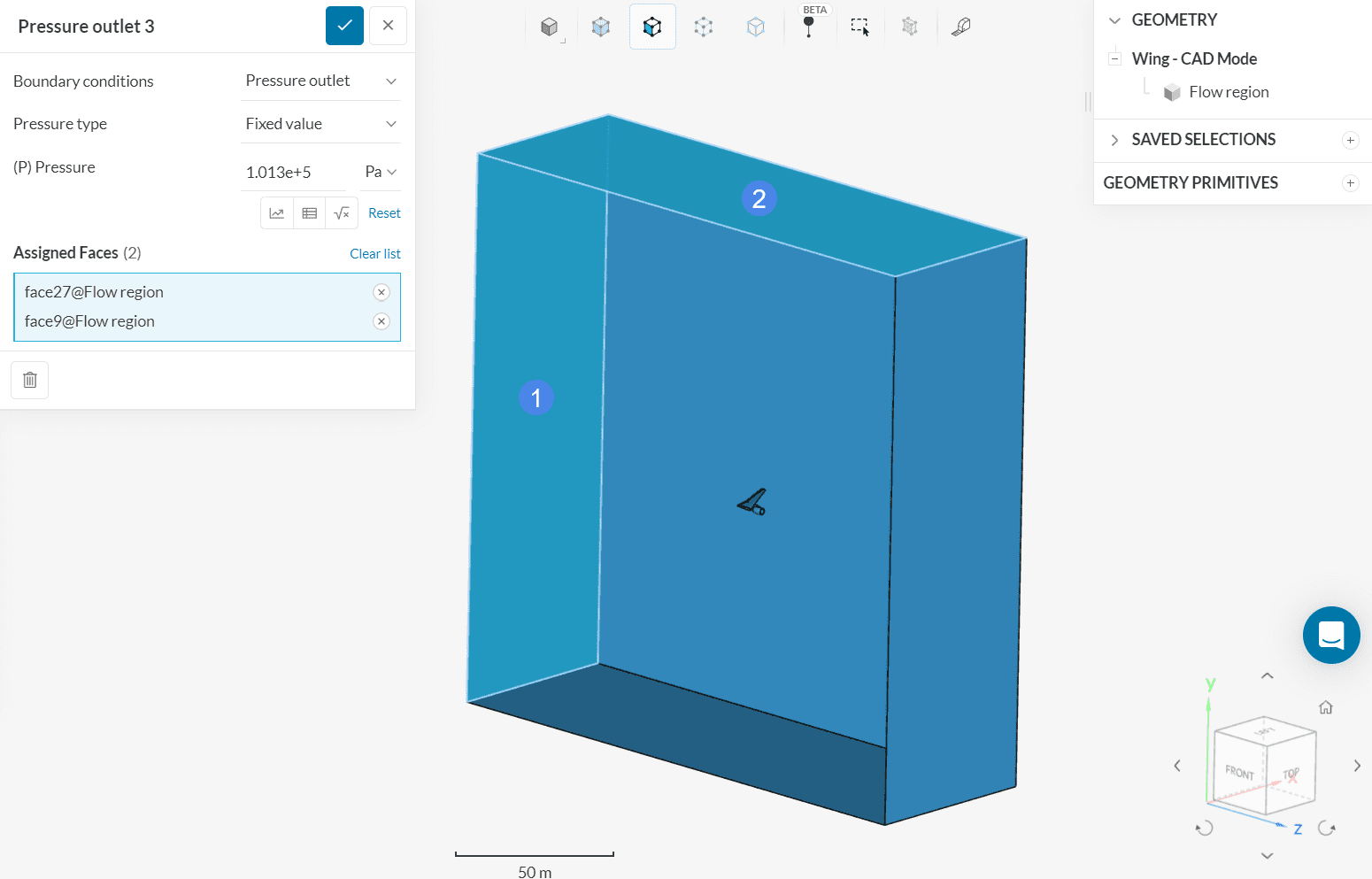
c. Pressure Outlet
Create yet another boundary condition. Select ‘Pressure outlet’ and assign the following enclosure faces to it:
d. Velocity Inlet
Due to the high velocities involved, compressible simulations require extra care during the setup phase. Aiming to improve stability in early iterations, the velocity will be ramped, starting from a magnitude of 11.6 m/s at iteration 0, to the final magnitude of 116 m/s at iteration 600.
Furthermore, an angle of attack of 3 degrees for the wing will be taken into account. Therefore, the velocity will have components in the Y and Z directions.
Create a ‘Velocity inlet’ boundary condition and follow the steps demonstrated in the picture:
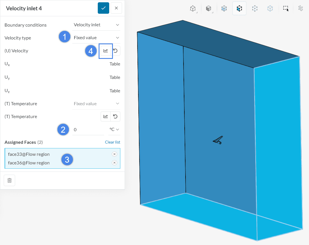
- Keep ‘Fixed value’ for (U) Velocity;
- Set Temperature to ‘0 °C’;
- Assign the inlet surfaces to the boundary condition;
- Click on the highlighted icon to access the velocity table and define it as pictured below:
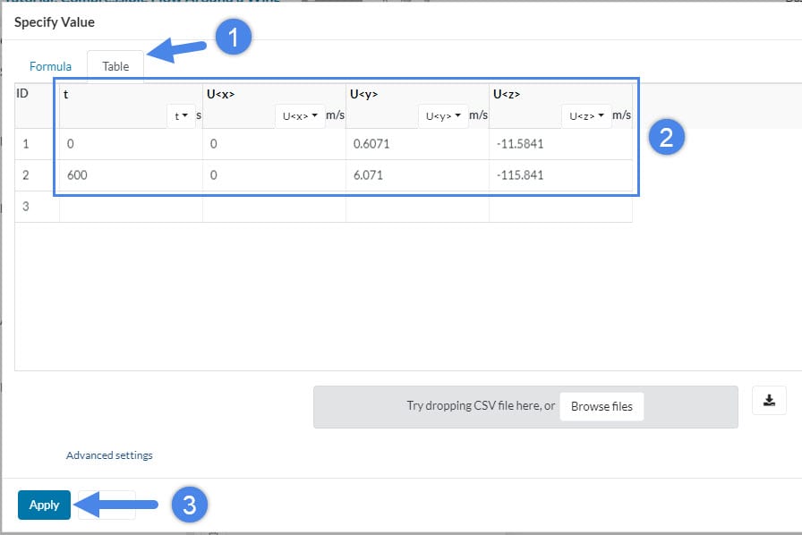
- Click ‘Table’ to access the table input.
- Define the ramp according to the table below.
- Confirm by hitting ‘Apply’.
| t | U<x> | U<y> | U<z> |
| 0 | 0 | 0.6071 | -11.5841 |
| 600 | 0 | 6.071 | -115.841 |
e. Walls – No-Slip
All solid walls should receive a no-slip condition. With this configuration, the velocity on the assigned entities is set to zero.
Saved selections help to assign a group of faces all at once. As we need all the faces of the wing to be modeled as physical walls, let’s group them as a saved selection.
To create saved selections for the wing walls, follow these steps:
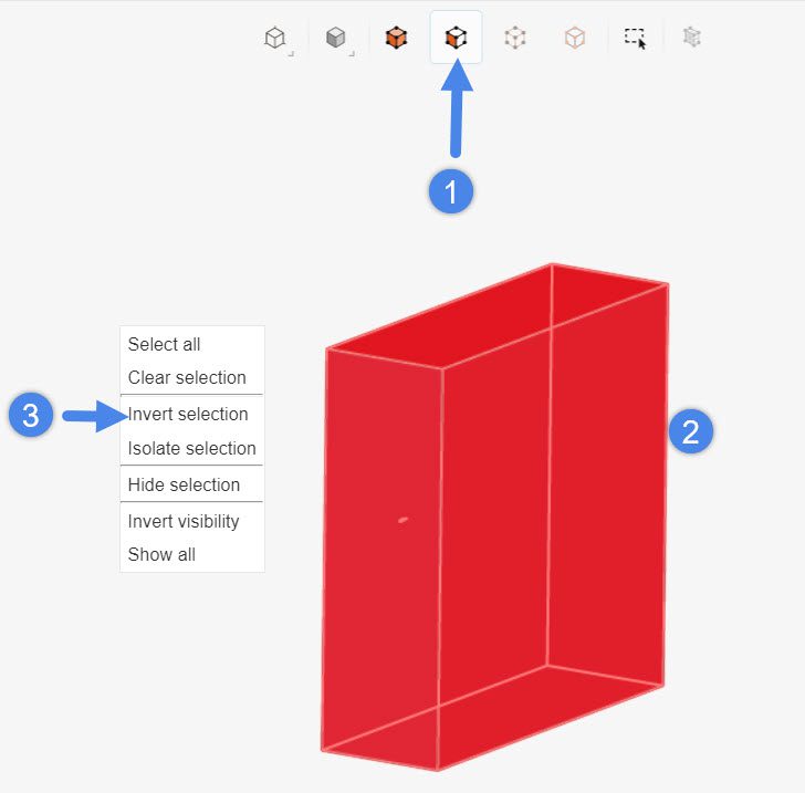
- Enable the select face mode in the viewer
- Select all 6 boundary faces of the enclosure
- Right-click in the viewer and ‘Invert the selection’
Now, all the walls of the wing are selected. Follow the instructions in the figure below to create the set:
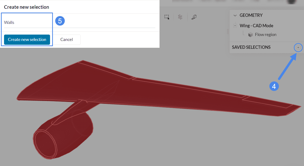
- 4: Click on the ‘+ button’ next to Saved Selections;
- 5: Name your newly created set appropriately. For example, as ‘Walls’ or ‘Wing surfaces’.
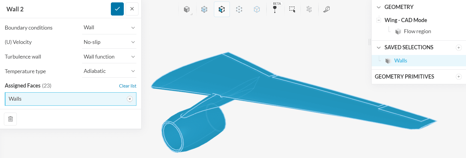
Now, create a wall boundary condition and assign it to the newly created set. Make sure to set ‘Adiabatic‘ for temperature.
Note
Check out this page, if you are interested in other boundary conditions available in SimScale.
2.3 Initial Conditions
The values for the initial velocity and temperature will require changes from the default. Doing this stabilizes the calculation.
The velocity field will receive the same initialization as the velocity inlet.
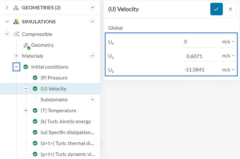
Did you know?
Initializing the velocity means that the air around the wing in our virtual wind tunnel is already moving.
If we would not predefine it, there would not be air movement at the beginning of the calculation and the solver would have to calculate it based on the specified inlet velocity.
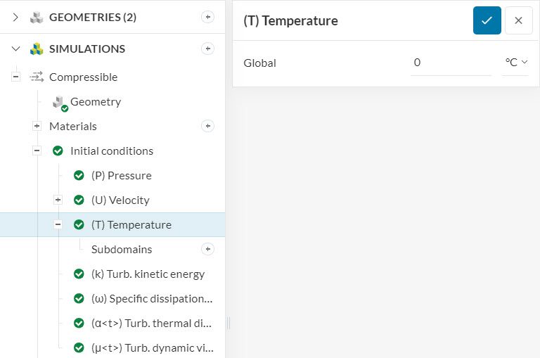
And, for temperature, please initialize the entire domain with 0 Celsius.
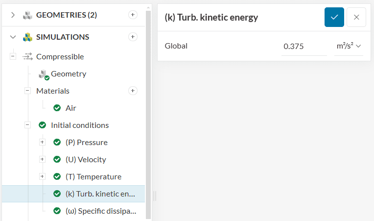
Set the initial turbulent kinetic energy to ‘0.375’ \(m^2/s^2\).
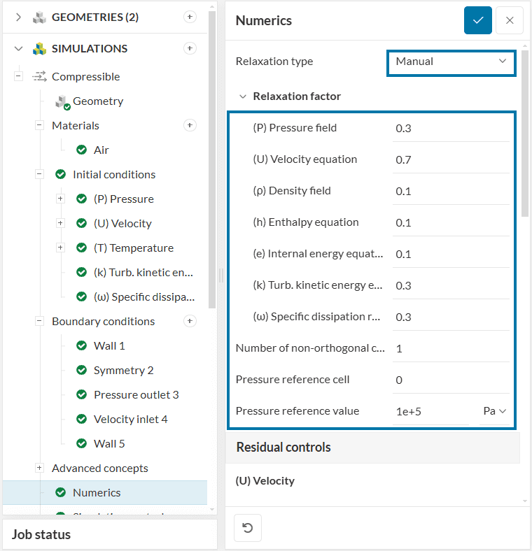
2.4 Numerics
In the Numerics tab, make sure the Relaxation type is Manual. Retain the values of the Relaxation factors as shown in Figure 26.
2.5 Simulation Control
Please set up the wing simulation control as shown below:
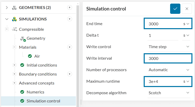
- Under Simulation control, define ‘3000’ iterations to End time and Write interval
- Also, raise the Maximum runtime to ‘30000’ seconds
For more information about the simulation control parameters, check this article.
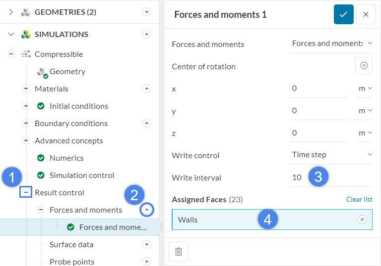
2.6 Result Control
By setting result controls, you can observe the convergence behavior of several parameters of interest. Hence it is an important indicator to evaluate the quality and trustability of the results.
The first result control to set is a Forces and moments control. Writing the forces data every 10 iterations is enough to assess convergence. Assign it to the ‘Walls’ saved selection:
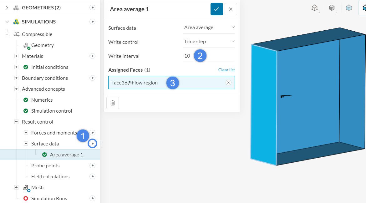
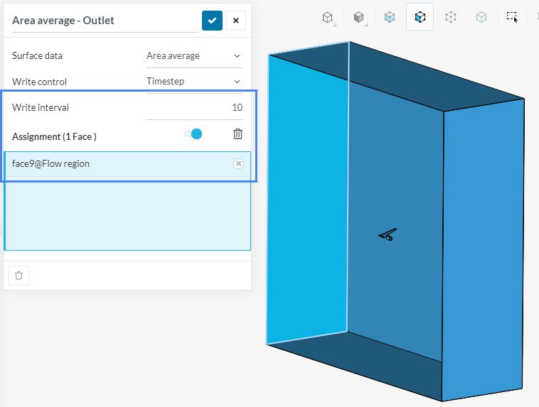
Now, click on the ‘+ button’ next to Surface data to create ‘Area averages’. A total of two controls will be created, one for the inlet and one for the outlet.
Similarly, for the main outlet:
3. Mesh
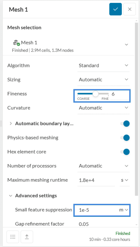
To create the mesh, we recommend using the Standard algorithm, which is a good choice in general as it is quite automated and delivers good results for most geometries.
From the main settings, increase Fineness to ‘6’ and in the advanced settings, set Small feature suppression to ‘1e-5’. Retain the default values for all the other settings.
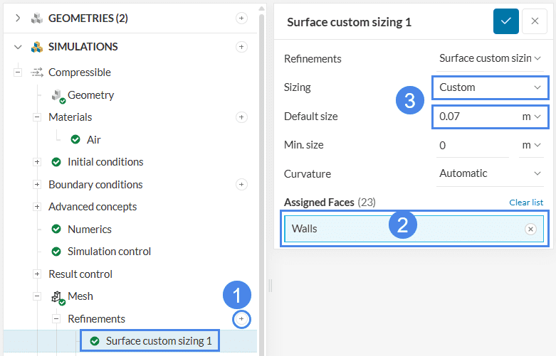
3.1 Surface Custom Sizing Refinement
Click on the ‘+ button’ next to Refinements. A ‘Surface custom sizing’ will be assigned to the ‘Walls’ saved selection. Set Sizing to ‘Custom’ and the Default size to ‘0.07’ meters:
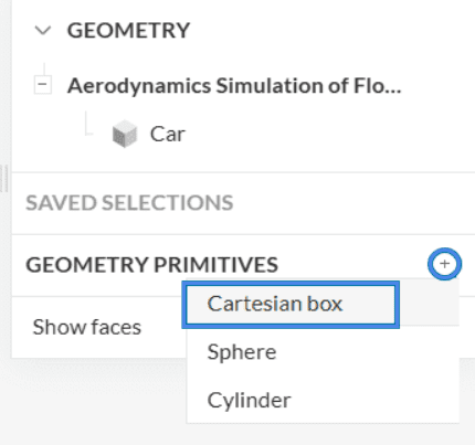
3.2 Creating Geometry Primitives
To add a volume refinement of a different size and dimension compared to the entire fluid domain, we can create and use Geometry Primitives. As fluid flows around a body, a turbulent region is developed downstream. This region is called Wake. Since gradients in the wake are often high, we shall refine the mesh in this region. Let us first create a Geometry Primitive that includes this region. In this case, we select to create a ‘Cartesian box’.
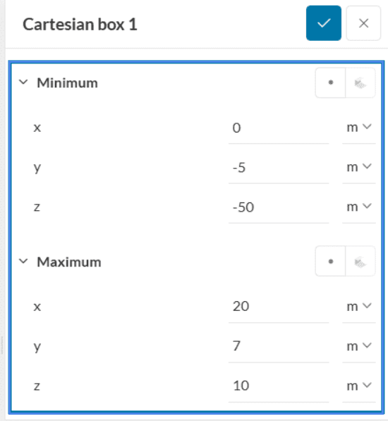
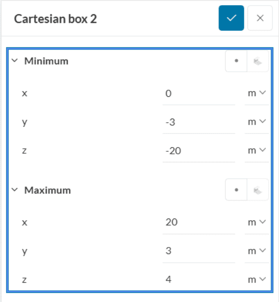
The following coordinates are used for this first cartesian box:
Similarly, we create a second geometry primitive. This is also a cartesian box but with the following coordinates:
The boxes are now used as volumes to refine the mesh in a Volume custom sizing refinement.
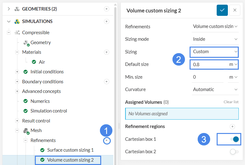
3.3 Volume Custom Sizing Refinement
First, create a new Volume custom sizing refinement. Specify Sizing as ‘Custom’ and set the Default size to ‘0.8’ meters and toggle on the ‘Cartesian box 1’ we created in the previous section.
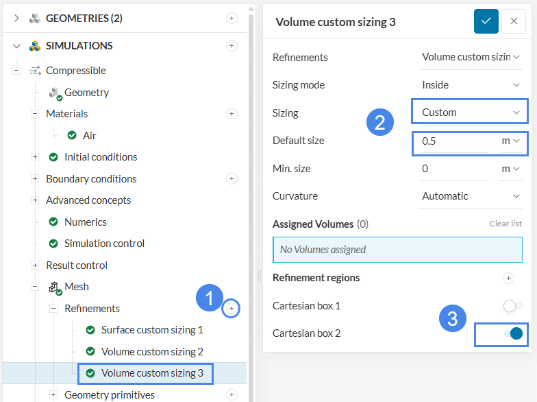
Following the same steps, create another volume custom sizing refinement. This time, set the Default size to ‘0.5’ meters.
3.4 Generating the Mesh
At last, head back to the main mesh settings and hit ‘Generate’.
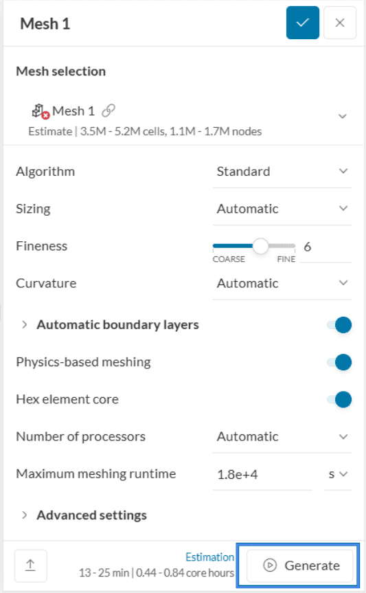
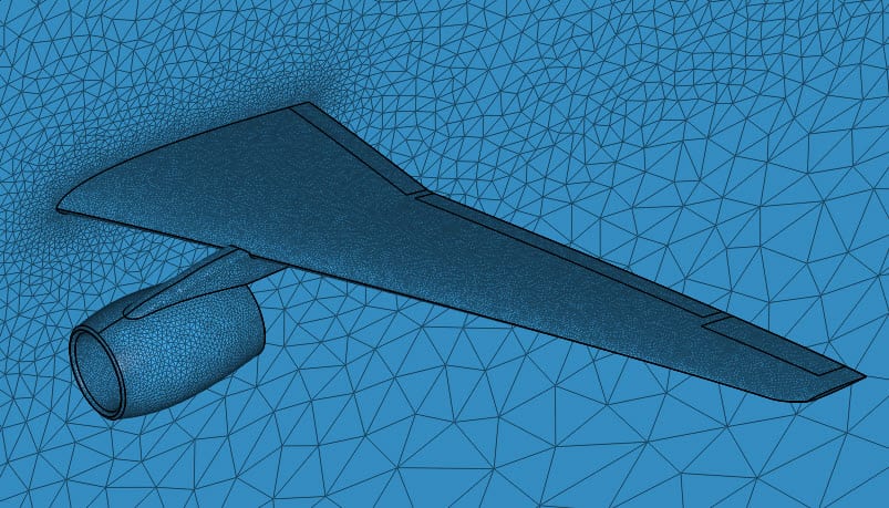
The resulting mesh takes about 10 minutes to complete. After the operation, the mesh looks like this around the wing:
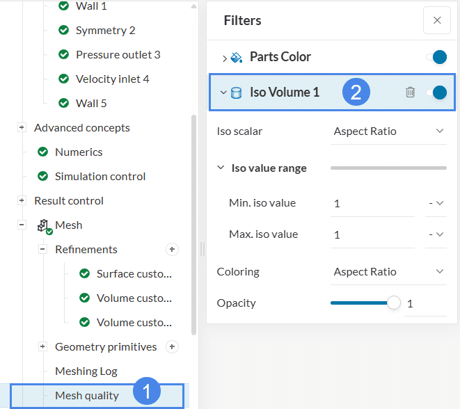
3.5 Mesh Quality Inspection
Within SimScale, it’s possible to visually inspect mesh quality parameters. Amongst the available quality parameters, we have non-orthogonality, aspect ratio, and volume ratio.
To access this feature, click on ‘Mesh quality’, which is located under Mesh. The post-processing environment then opens up. A particularly helpful filter is Iso Volumes.
By playing with the minimum and maximum iso values, it’s easy to identify bad cells. For example, Figure 41 shows the cells in the mesh, within the specified range of values, according to ‘Non-orthogonality’. Please note that the default iso values in your mesh may be different since the meshing algorithm is constantly being updated.
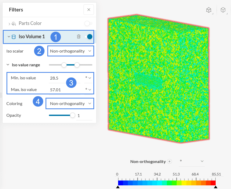
A visual representation of mesh quality is extremely helpful when trying to improve the mesh. For our mesh, the maximum observed value for the non-orthogonality is around 85, which is acceptable. Therefore, we can proceed to run the simulation.
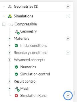
4. Start the Simulation
Click on the ‘+ button’ next to Simulation Runs and ‘Start’ the process.
While it’s running, you can access the intermediate results by clicking on ‘Solution Fields’. They’re updated as the iterations go by!
The entire simulation takes between 1 to 2 hours to finish, depending on the number of processors. In the reference project, which is linked below, we calculated a few more iterations, to assure complete convergence.
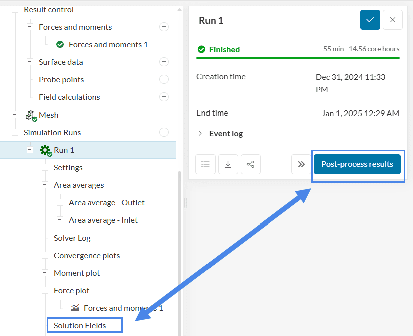
5. Post-Processing
After the simulation is finished, you can expand Run 1 to check the results.
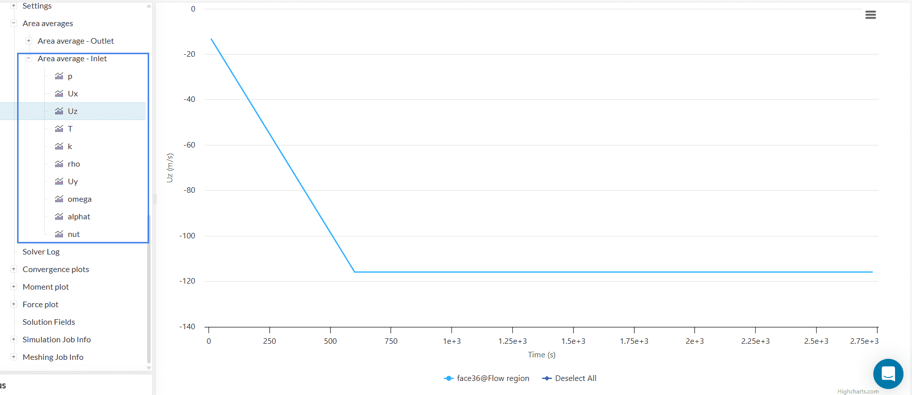
5.1 Result Controls
Once the run is finished, open the area average at the inlet result control. By inspecting Uz and Uy, the velocity ramping is clearly appreciated:
For any wing simulation, force plots are commonly used to assess convergence. By inspecting the force plot from this simulation, we can see that all parameters converge nicely:

For compressible external aerodynamics simulations, other parameters useful to assess convergence are:
- Inlet: pressure.
- Outlet: temperature, velocities, and density.
5.2 Surface Visualization
For further post-processing click on the ‘Post-process results’ or the ‘Solution Fields’ button.
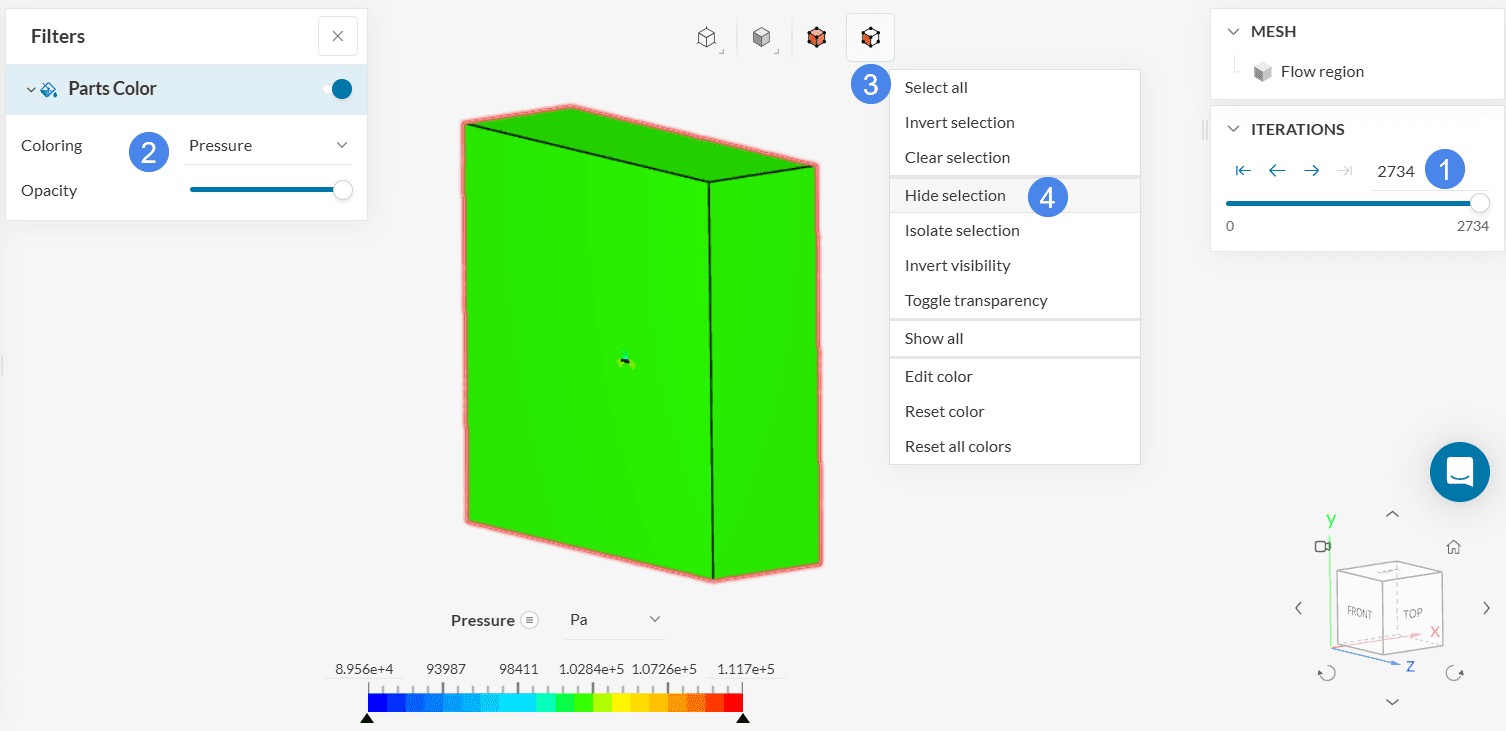
- Make sure the post-processor shows the results for the final time step;
- Go to the Parts Color and choose ‘Pressure‘ from the Coloring drop-down menu. Feel free to change the parameter if you wish;
- Click on the 6 faces of the enclosure, then right-click on the viewer
- Select the ‘Hide selection’ option, to reveal the surface of the wing:
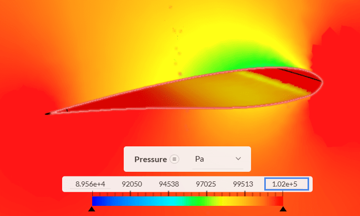
Make sure to right-click on the color scale at the bottom of the screen and select the ‘Use continuous scale’, for a smoother transition between color contours:
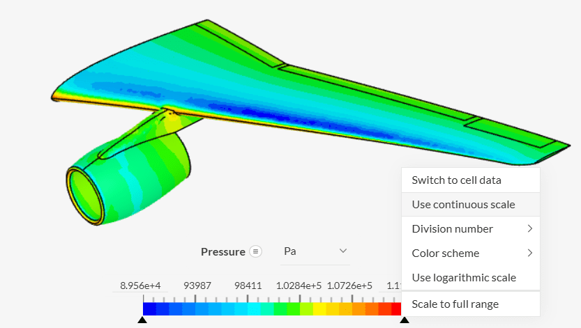
The tip of the plane exposed to the freestream velocity has the highest pressure values. On the contrary, the upper side of the wing has a low-pressure distribution, as expected for a lift-generating device.
This is how the results will appear if you set visible only the symmetry plane, and apply a value of ‘1.02e5 \(Pa\)’ as the upper limit of the legend at the bottom:
5.3 Streamlines
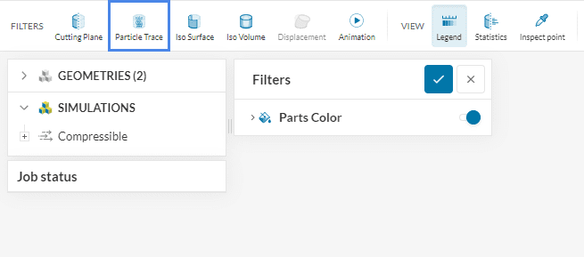
For streamline visualization, select the ‘Particle Trace’ filter from the top bar:
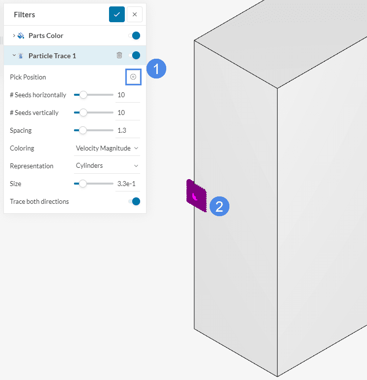
- Click on the circle icon next to the Pick Position;
- Apply the seed point on the inlet face, as close to the symmetry face and the center of the y-axis as possible. Use a translucent render mode if needed in order to align the seed point with the wing.
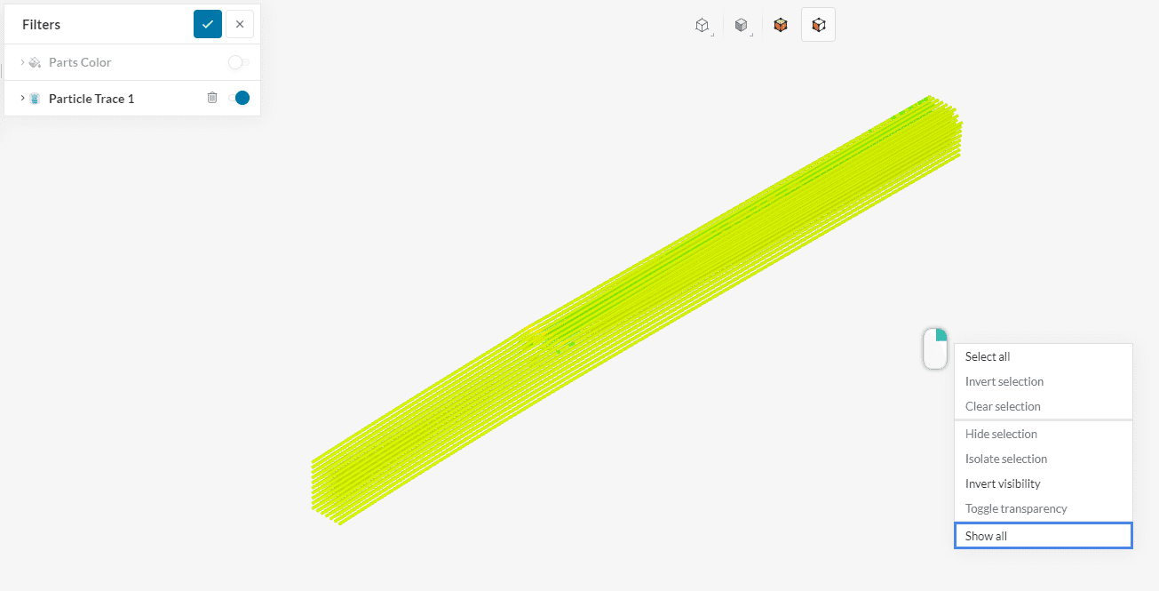
Only the streamlines will be visible after applying the filter. Collapse the Particle Trace 1 tab, right-click on the workbench, and choose the ‘Show all’ option:
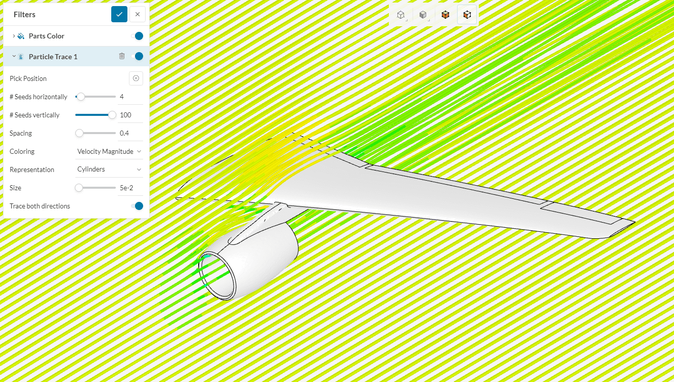
Proceed to select all six faces of the domain and hide them, like in Figure 46, so only the wing surface is visible apart from the streamlines. Go back to the Particle Trace tab, and modify the settings as follows:
- The # Seeds horizontally represents the number of streamline rows along the z-axis. Set it to ‘4’. The # Seeds vertically represents the number of rows along the y-axis. Make sure it is big enough that it covers the whole y dimension of the domain. An input of ‘100’ should be fine for this case;
- Set the Spacing distance between streamlines to ‘0.4’;
- Select ‘Velocity Magnitude’ as Coloring;
- You can control the diameter of the cylinders with the Size option. Set it to ‘5e-2’;
- For this case, you can have the Trace both directions option disabled, as the flow here travels from the inlet only towards the positive x-direction.
With these settings, this is how the streamlines will finally appear:
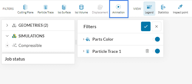
5.4 Animation
Animations can be created by choosing ‘Animation’ from the top bar:
Switch the Animation type to ‘Particle Trace’:
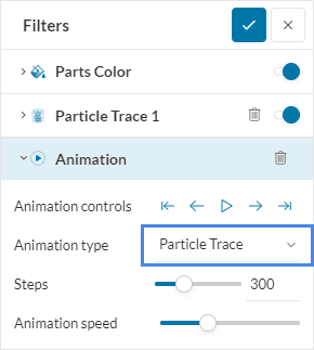
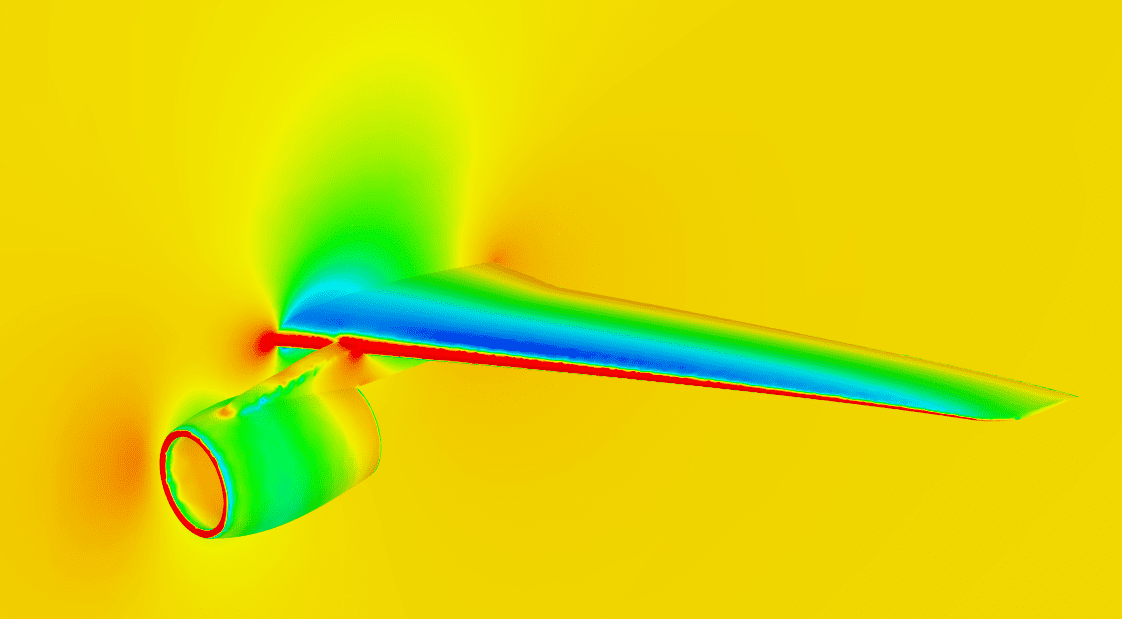
Click the play button to start the animation. Below is an example of animating the streamlines, colored with the velocity magnitude, during the final time step:
As a result of lift generating airfoils used in airplane wings, it can be seen that the top surface has higher velocity due to curvature.
Analyze your results with the SimScale post-processor. Have a look at our post-processing guide to learn how to use the post-processor.
Congratulations! You finished the tutorial!
Last updated: April 4th, 2026
Did this article solve your issue?
How can we do better?
We appreciate and value your feedback.


