What is Turbulent Flow?
In fluid dynamics, a turbulent flow refers to an irregular flow in which eddies, swirls, and flow instabilities occur. It is governed by high-momentum convection and low-momentum diffusion. It is in contrast to the laminar regime, which occurs when a fluid flows in parallel layers with no disruption between the layers.
The turbulence regime is extremely frequent in natural phenomena and engineering applications; some examples are the rise of cigarette smoke, waterfalls, blood flow in arteries, and most of the terrestrial atmospheric recirculation.
In terms of engineering applications, the turbulent regime occurs in the aerodynamics of all vehicles such as cars, planes, and ships; but also in many industrial applications such as heat exchangers, quenching processes, or continuous casting of steel — applications where higher Nusselt numbers indicate enhanced convective heat transfer.
Structure of Turbulent Flow
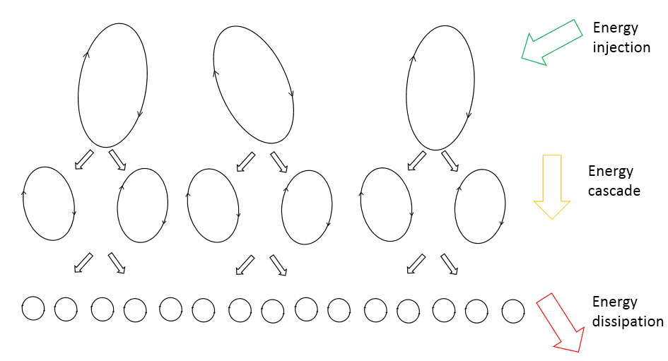
In 1920, Lewis Fry Richardson summarized his works about the structure of turbulence for meteorological applications through a celebrated rhyme published in Weather Prediction by Numerical Process\(^1\):
“Big whirls have little whirls that feed on their velocity, and little whirls have lesser whirls and so on to viscosity”\(^1\)
This principle was motivated by energetical considerations; big eddies are highly inertial and tend to be unstable. Their motion feeds smaller eddies thanks to a local transfer of kinetic energy. These smaller eddies undergo the same process, giving rise to even smaller eddies that inherit the energy of their parent eddy, and so on.
This transfer of energy is usually called “energy cascade” and it is mainly inertial, thus almost no energy dissipation occurs until reaching a sufficiently small length scale such that the viscosity of the fluid can effectively dissipate the kinetic energy. This process has been depicted in Figure 1.
Richardson’s studies highlight an essential feature of turbulent flows: they are energy-demanding. A turbulent flow will dissipate energy and decay to a laminar flow at the smallest scales unless it is fed by an external source of energy.
Smallest Turbulence scales
The complexity of turbulence and its aleatory behavior led scientists to use statistical models to describe turbulence flows.
In 1941, Kolmogorov enhanced Richardson’s theory \(^2\). Kolmogorov postulated that for a high enough Reynolds number, the small-scale eddies are isotropic, while large eddies may be anisotropic (or anyway, dependent on the specific domain’s topology).
This assumption is critical because it means that the statistical analysis of small eddies is independent of any specific geometry and thus it is universal for all turbulent flows. Under this hypothesis, Kolmogorov statistically described the main features of the smallest turbulence scale (known as “Kolmogorov microscales”) as follows:
| Kolmogorov length scale | \(\eta = \left(\frac{\nu^3}{\epsilon}\right)^{0.25}\) |
| Kolmogorov time scale | \(\tau=\left(\frac{\nu}{\epsilon}\right)^{0.5}\) |
| Kolmogorov velocity scale | \(u=\left(\nu\epsilon\right)^{0.25}\) |
where:
- \(\nu\) is the kinematic viscosity
- \(\epsilon\) is the turbulence kinetic energy
- \(\eta\) ,\(\tau\) and \(u\) are the characteristic length, period (or “turnover time”) and velocity of the smallest eddies respectively
Reynolds Number
The real onset of scientific studies on turbulence can be found in the work of Osborne Reynolds in the second half of the 19\(^{th}\) century. Through experimental investigations, Reynolds showed the transition between a laminar and a turbulent regime. He also suggested that this transition was directly linked to the ratio between inertial and viscous forces. This ratio was computed by George Gabriel Stokes in 1851 and has been named “Reynolds number” in honor of Osborne Reynolds, who popularized it.
This dimensionless number is defined as:
$$ Re = \frac{\rho ud}{\mu}=\frac{ud}{\nu} \tag{1}$$
where:
- \(\rho\) is the density of the fluid
- \(u\) is the macroscopic velocity of the flow
- \(d\) is the characteristic length (or hydraulic diameter)
- \(\mu\) is the dynamic viscosity of the fluid
- \(\nu\) is the kinematic viscosity of the fluid.
Turbulent flows occur when \(Re\) exceeds a certain threshold (dependent on the application’s topology and flow physics) called “Critical Reynolds number”.
Turbulence Modeling in CFD
The main equations that dictate the fluid motion are composed of the application of the conservation laws, and these equations are called the Navier-Stokes Equations (NSE). The motion of the fluid is fully described by the NSE whether the flow is laminar or turbulent. Below, their incompressible form is provided which allows modeling the fluid motion:
$$ \rho\partial_tu_i+\rho u_ju_{i,j}=-\rho p_{,i}+\mu u_{i,jj} \tag{2}$$
$$ u_{i,i}=0 \tag{3}$$
Where
- \(u\) is the velocity
- \(p\) is the pressure of the fluid
- \(\rho\) is the fluid’s density
- \(\mu\) is the fluid’s dynamic viscosity
The NSE are inherently very difficult to solve due to its non-linear nature, which mainly stems from the convective acceleration term \(u_ju_{i,j}\). Therefore, different methodologies were developed to allow for a numerical solution with appropriate initial and boundary conditions by discretizing the fluid domain.
Overview of Turbulence Modeling Methods
There are multiple approaches to the modeling of turbulence in CFD; they are mainly characterized by the mesh resolution of the problem, which in return defines the computational power needed for a simulation.
Direct Numerical Simulation (DNS)
A very high-resolution mesh that can resolve the turbulent flow’s smallest spatial and temporal scales is called a Direct Numerical Simulation (DNS). The structure of the turbulence in DNS is totally represented. However, the computational cost associated with DNS is extremely high. Thus, DNS is limited to small-scale problems with low Reynolds numbers \(^3\).
Large Eddy Simulation (LES)
In a Large Eddy Simulation (LES) turbulence model, the smallest scales of turbulence are spatially filtered out to be modeled. While the largest, most energy-containing scales are resolved directly by the mesh. This approach allows for having a coarser mesh resolution than in DNS and hence making this method to be more universal and applicable to various fluid flow problems.
SimScale offers three LES turbulence models, namely: LES Smagorinsky, LES Spalart-Allmaras, and LES Smagorinsky direct (available only for the Incompressible LBM solver)
Detached Eddy Simulation (DES)
Detached Eddy Simulation turbulence models combine the methodology from both RANS and LES models. In the region near the wall where the turbulence length scales are smaller than the maximum grid size, the DES model assigns a RANS model to that region. Consequently, in regions where the turbulent length scales are larger than the maximum grid size the DES model assigns an LES model to that region. This approach allows for reducing the computational cost associated with the simulation since the grid resolution does not need to be as demanding as a pure LES simulation.
SimScale offers two DES turbulence models in the Incompressible LBM solver, namely:
‘K-omega SST DDES’ and ‘K-omega SST IDDES
Reynolds Averaged Navier-Stokes (RANS)
Another much less computationally demanding method is the Reynolds-Averaged Navier-Stokes (RANS). It uses a time-averaged solution of the flow fields. The Reynolds averaging process introduces an additional term to the NSE known as Reynolds stress.
Let’s consider again the NSE for an incompressible Newtonian fluid:
$$ \rho\partial_tu_i+\rho u_ju_{i,j}=-\rho p_{,i}+\mu u_{i,jj} \tag{2}$$
$$ u_{i,i}=0 \tag{3}$$
The principle is to consider the flow as the sum of mean flow and turbulent/unsteady flow. The steady mean velocity can be computed as the Favre average of the global velocity:
$$ U_i=\lim_{T\rightarrow\infty}\frac{1}{T}\int_0^Tu\: dt \tag{4}$$
thus, the velocity can be decomposed as:
$$ u_i=U_i+u’_i \tag{5}$$
where \(U\) is the mean velocity and \(u’\) is the turbulent flow velocity (or turbulent scales). \(T\) is the averaging time scale, which must be small enough to have a good approximation of the problem, but also sufficiently higher than the turbulence time scale, i.e. the Kolmogorov’s turnover time. By substituting the averaged quantities in the Navier-Stokes equation, we obtain the RANS equations:
$$ \rho U_j U_{i,j} =-\rho P_{i} +\mu U_{i,jj} -\left( u_{i}’ u_{j}’\right) _j \tag{6}$$
$$ U_{i,i}=0 \tag{7}$$
where \(\left( u_{i}’ u_{j}’\right) _j\) is usually called “Reynolds stress” and represents the effect of the small-scale turbulence on the average flow. The RANS equations have no unique solution because they are not in a close form, the unknowns being more than the equations. Thus, additional equations are needed to close the problem. The most common strategy used in CFD is to relate the Reynolds stress to the shear rate by the Boussinesq relationship:
$$ u_i’u_j’=2\frac{\mu_t}{\rho}S_{ij} \qquad with\qquad S_{ij}=\frac{1}{2}\left(U_{i,j}+U_{j,i}\right) \tag{8}$$
Where \(\mu_t\) is the turbulent viscosity, which is usually computed from the turbulence models\(^4\).
SimScale offers three turbulence models from the RANS family, namely: K-epsilon, K-omega, K-omega SST
Now that we understand the basic concept of various turbulence modeling approaches, we can complement that with a qualitative visual description as shown in figure 2. It illustrates the extent to which the turbulence scales can be observed when comparing DNS, LES, and RANS.
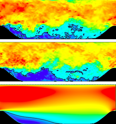
Bottom: RANS ; Middle: LES ; Top: DNS
RANS, LES, and DES
SimScale offers simulation with a variety of turbulence models to choose from the family of RANS, LES, DES. Choose between a Community or a Professional account and start simulating.
Applications of Turbulent Flow
Turbulent flows are present in many natural phenomena (e.g. river flows, atmospheric streams, natural convection) and engineering applications (e.g. wind flow in a city, aerodynamic analyses, continuous casting, quenching process, cooling/heating systems).
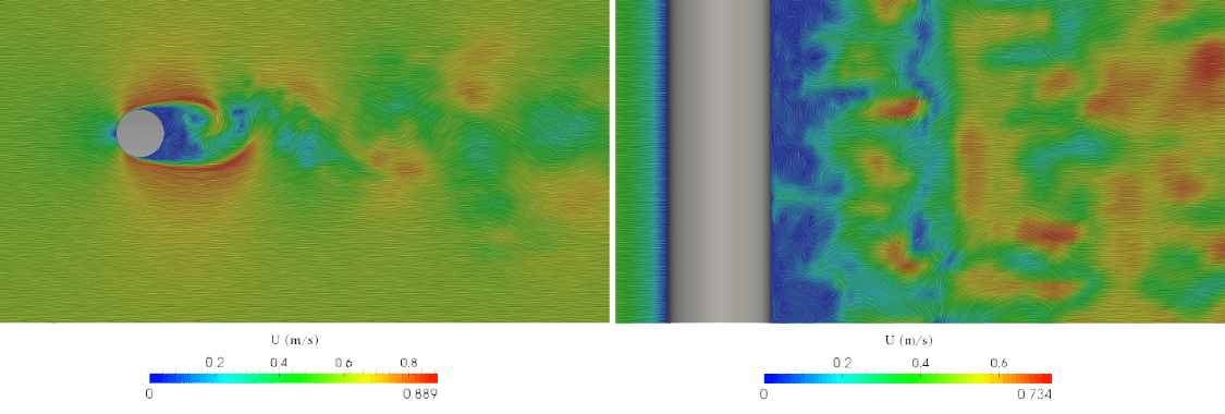
In this section, two small applications done using SimScale have been reported. The first (Figure 3) is an analysis of the flow around a cylinder. The case can be applied to the flow of a river around a bridge column, but it also has great academic value since it is a widely used benchmark for validation.
Furthermore, it is often used to show the different regimes (linked to the presence, size, and frequency of eddies) at different problem configurations.
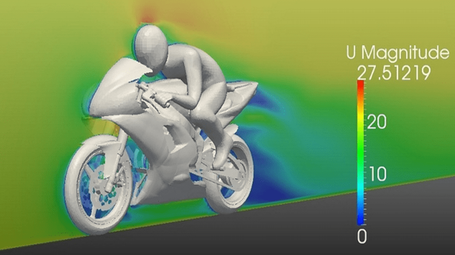
The second case is the aerodynamic analysis of a motorbike with a rider (Figure 4). The high velocities and the low viscosity of air encourage the development of a turbulent regime. Even if it is avoided as much as possible in order to reduce the drag linked to the detachment of eddies behind the vehicle.

References
- Richardson, L. F. Weather Prediction by Numerical Process (Cambridge Univ. Press, 1922)
- https://micropore.wordpress.com/2010/08/21/kolmogorov-originl-paper-on-turbulence/
- David C Wilcox et al. Turbulence modeling for CFD, volume 2. DCW industries La Canada, CA, 1998.
- https://www.cfd-online.com/Wiki/Turbulence_modeling
- M. Manhart. Turbulence modeling ss21, introduction to turbulence, 2021.
Last updated: March 16th, 2026
Did this article solve your issue?
How can we do better?
We appreciate and value your feedback.
What's Next
Compressible Flow vs Incompressible Flow

