Tutorial: Aerodynamics Simulation of Flow Around a Vehicle
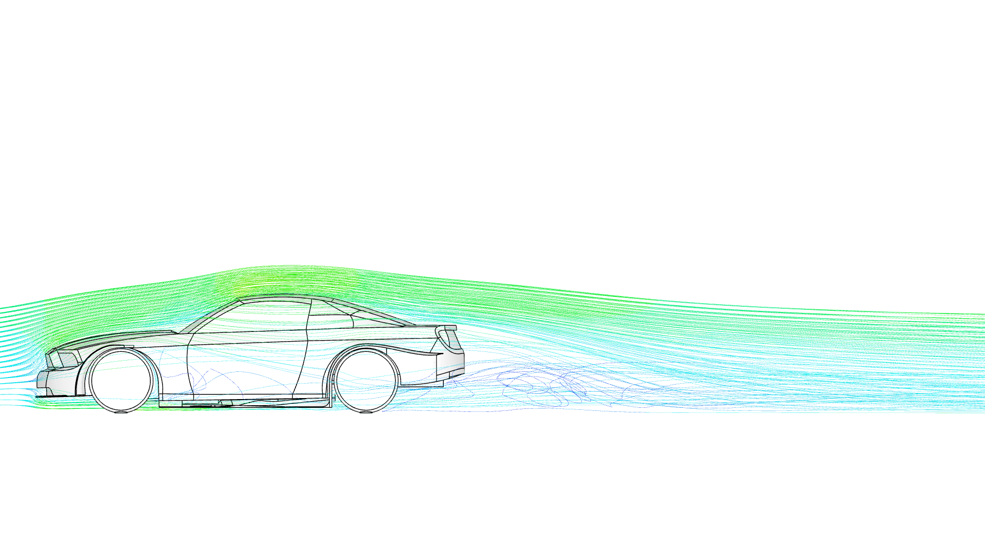
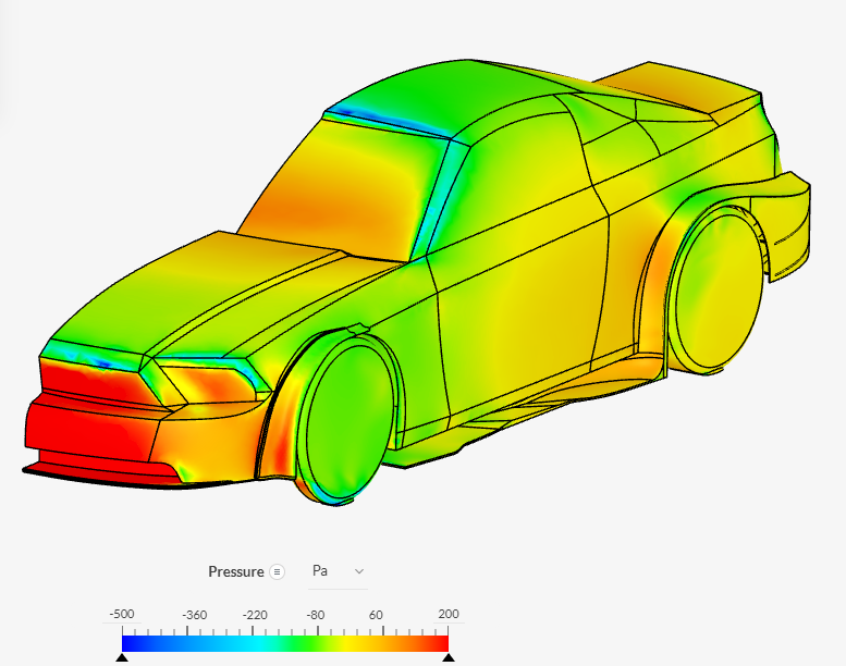
This tutorial shows how the aerodynamics of a vehicle can be analyzed by setting up an incompressible turbulent airflow around a moving vehicle. Figure 1 shows an example of the resulting flow behavior:
This tutorial teaches how to:
- Set up and run an incompressible simulation;
- Assign saved selections;
- Assign boundary conditions, material, and other properties to the simulation;
- Mesh with the SimScale standard meshing algorithm.
We are following the typical SimScale workflow:
- Prepare the CAD model for the simulation;
- Set up the simulation;
- Create the mesh;
- Run the simulation and analyze the results.
1. Prepare the CAD Model and Select the Analysis Type
1.1. Import the CAD into Your Workbench
The first step is to click on the button below. It will copy the tutorial project containing the geometry into your Workbench.
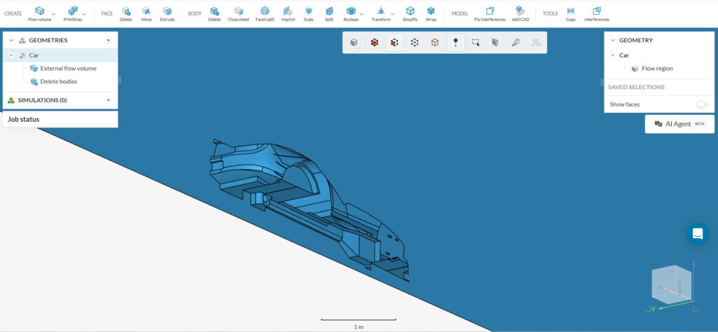
Figure 2 demonstrates what should be visible after importing the tutorial project:
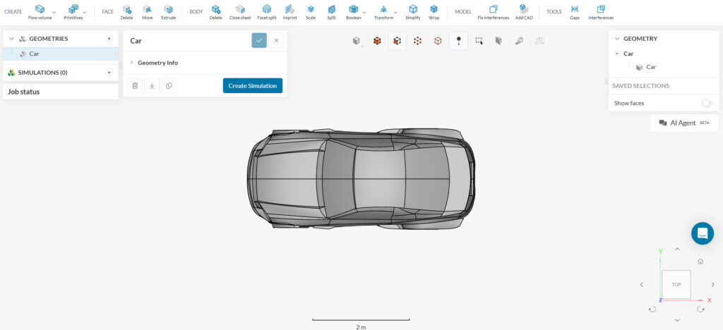
Note that the car geometry is not too detailed. Small and detailed features that don’t greatly affect aerodynamics, such as bolts and windshield wipers, should be removed or simplified.
With this approach, the computation effort necessary throughout the entire simulation process can be reduced, while still obtaining meaningful results. Find more information about CAD preparation on this documentation page.
Did you know?
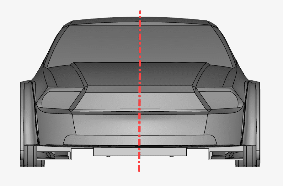
We can use the car’s symmetrical shape in our favor. As we expect the flow field to be mirrored along the symmetry plane of the car, we only need to use one half of the geometry. As a result we reduced the size of the flow region and the simulation will run faster, as only half of the cells are needed.
Crosswind Simulations
Note that the symmetry assumption does apply to analyses where the vehicle is traveling in a straight line with no crosswind. For crosswind analyses or cornering situations where the flow is oblique relative to the vehicle, a full vehicle analysis is required.
1.2. CAD Editing
The first step for this simulation is the creation of the fluid region. This will be the flow domain that will be used for the external aerodynamic analysis. For the incompressible analysis type, only the fluid region is used. To modify a CAD model, simply select the geometry from the list—the available CAD operations will then appear in the top toolbar. You can either work directly on the original model or create a duplicate and apply your changes to the copy. Eventually, the geometry of the car will be discarded, so only the flow region remains.
The External option is used to create the flow region around the model. Select ‘External’ next to Create, at the top left of the interface.
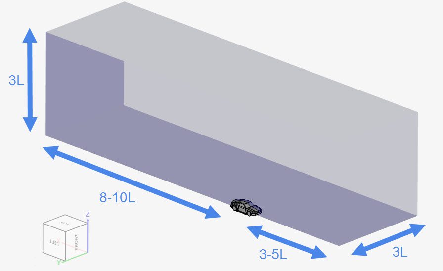
The dimensions of the flow region are chosen according to the length (L) of the vehicle. As a rule of thumb, the following values can be used:
- Downstream: ‘8-10’ times the length of the vehicle;
- Upstream: ‘3-5’ times the length of the vehicle;
- As much as necessary to the minimum z-direction, so that the ground can be tangent to the wheels;
- Other directions: ‘3’ times the length of the vehicle.
To further simplify the simulation the symmetric shape of the car is used to reduce the size of the flow domain. Set up the flow region dimensions in meters as shown below:
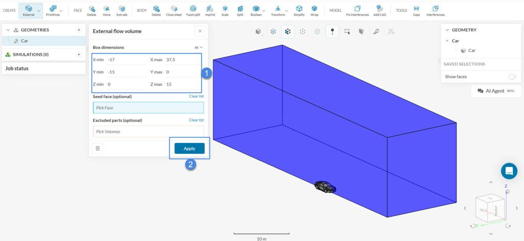
- X min: ‘-17.5’ \(m\)
- Y min: ‘-15’ \(m\)
- Z min: ‘0.0’ \(m\)
- X max: ‘37.5’ \(m\)
- Y max: ‘0’ \(m\)
- Z max: ’15’ \(m\)
After you are done, click ‘Apply’. Then select the ‘Delete’ feature next to the BODY section, to remove the ‘Car’ solid part:
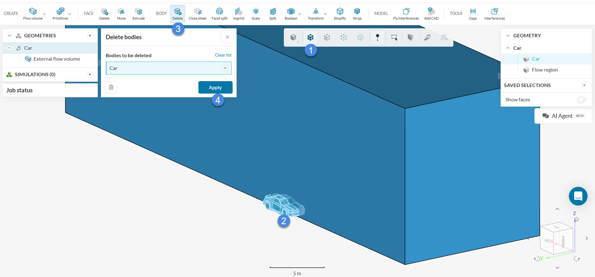
Select ‘Car’ from the Geometry tree at the top right and click ‘Apply’.
When the operation is finished and the car body is removed successfully, all the changes done will be applied to the originally imported geometry unless a duplicate of the model is being worked on.
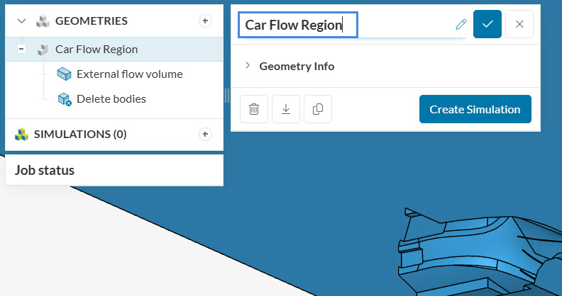
After the changes, for better clarity, rename the old geometry as ‘Car Flow Region’:
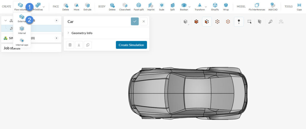
1.3 Create the Simulation
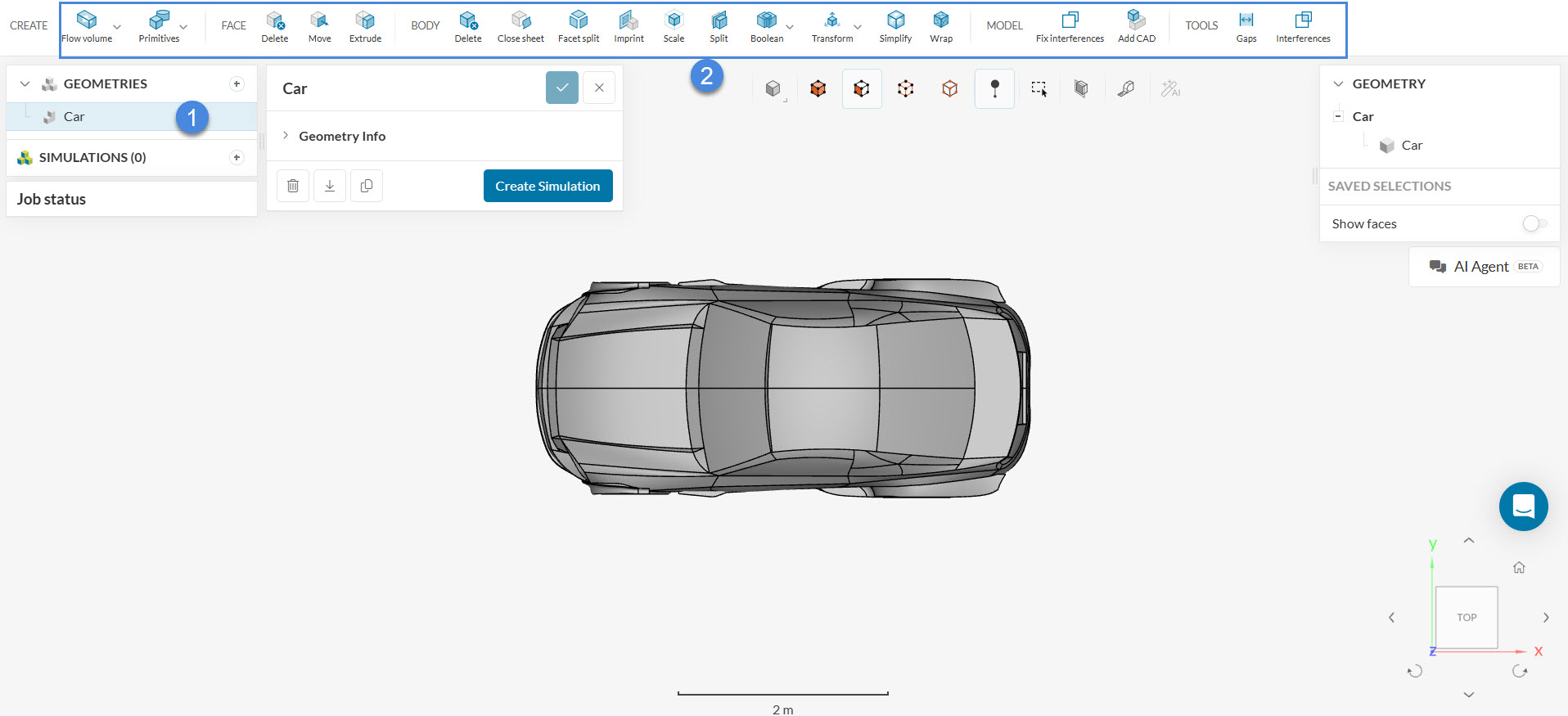
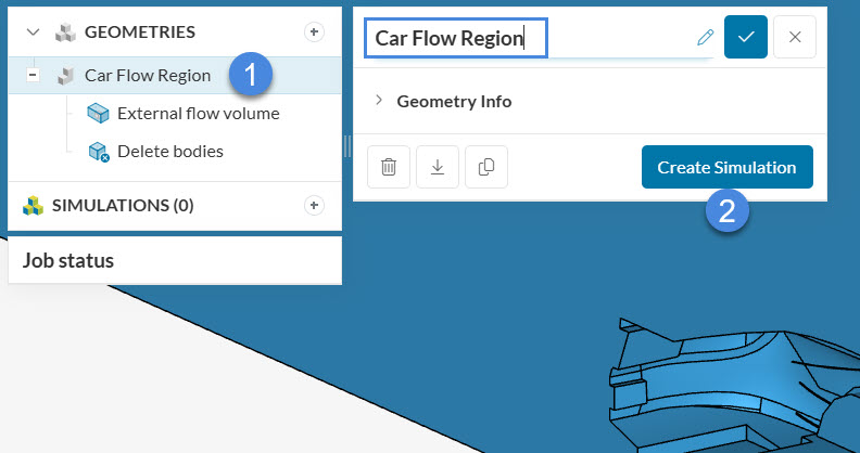
To start the simulation setup process, select the CAD ‘Car Flow Region’ and click on the ‘Create Simulation’ button.
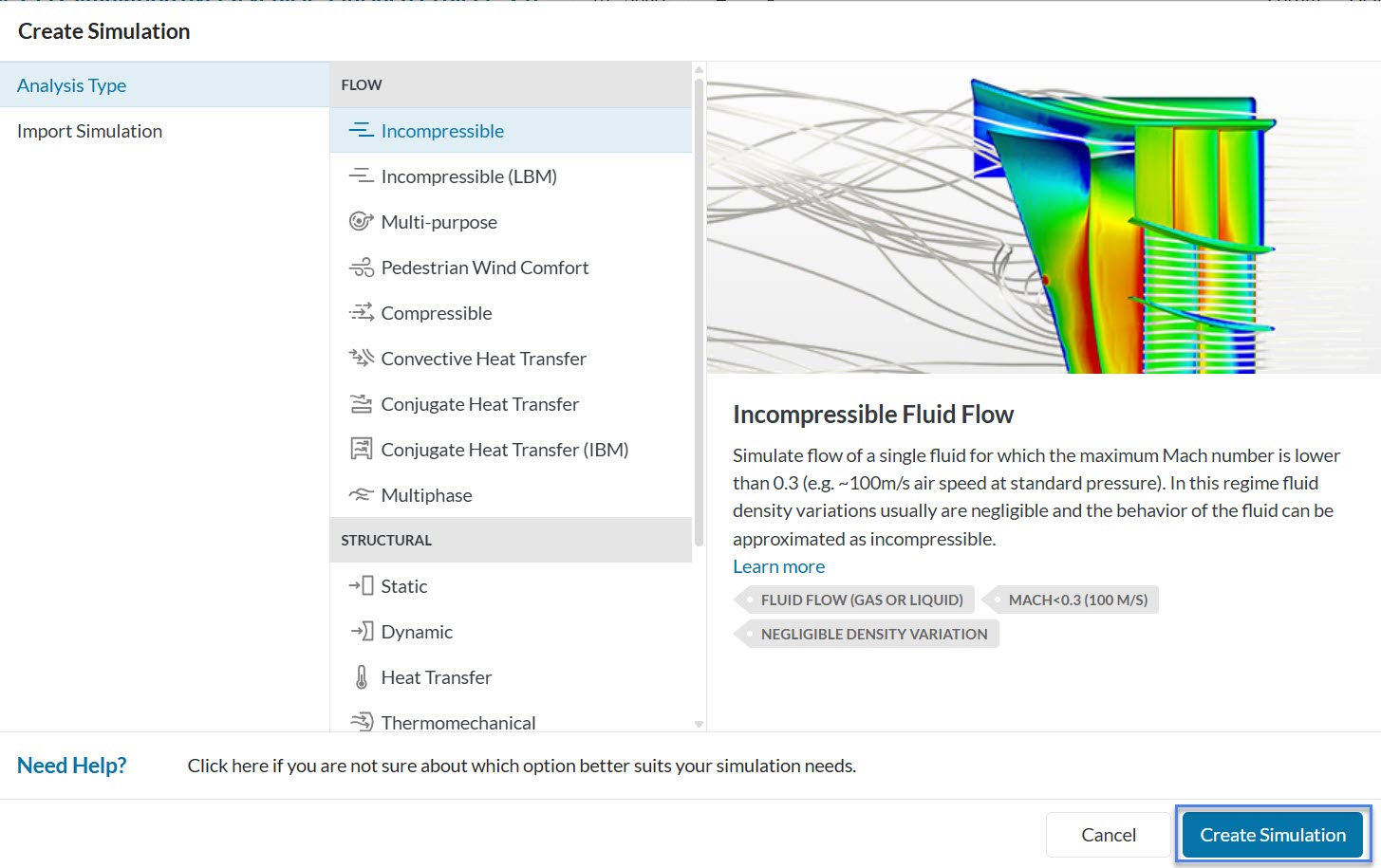
Doing so opens the analysis type choice widget. Choose ‘Incompressible’ as the analysis type. It can be used for cases where the Mach number remains lower than 0.3 in the entire domain, which will be the case for this tutorial. Proceed by clicking on the ‘Create Simulation’ button.
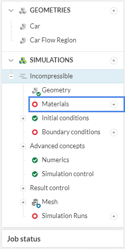
The simulation tree will be visible on the left-hand side of the interface. We have to set up all entries to be able to run the simulation. The global settings of the simulation remain as default:
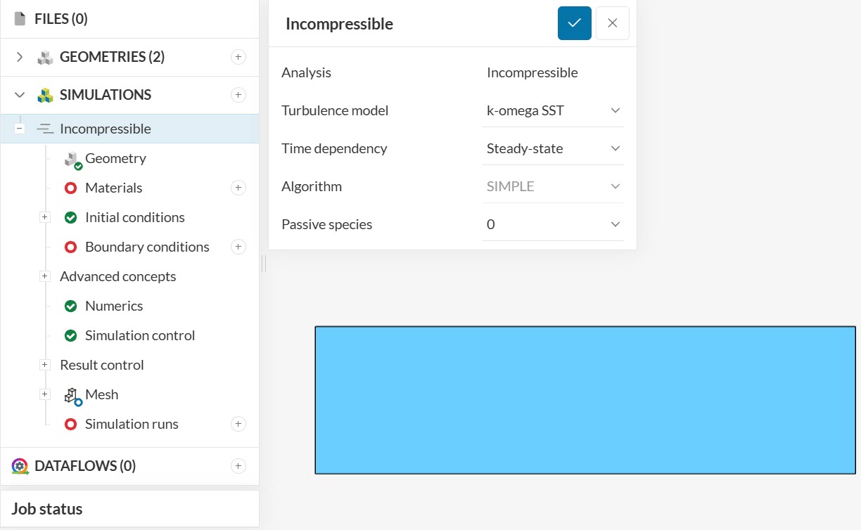
In this tutorial, we want to calculate the steady-state solution, which is independent of time. SimScale also supports transient analysis, which allows the calculation of time-dependent results.
Did you know?
The k-omega SST turbulence model is recommended for external aerodynamics cases.
It works as a blend between the k-omega and k-epsilon models. The k-omega model is predominant in the near-wall, switching to the k-epsilon model in the free-stream.
Find more information about the k-omega SST model in this documentation page.
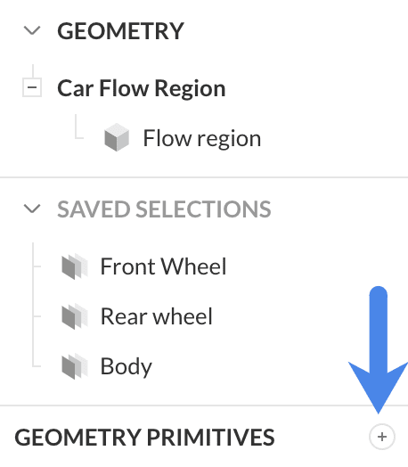
1.4 Create Saved Selection
Saved Selections are groups of faces. They are particularly helpful when the same group of faces is used several times during the simulation setup. The user can quickly select a given group of saved selections at once whenever they need to be assigned to a condition.
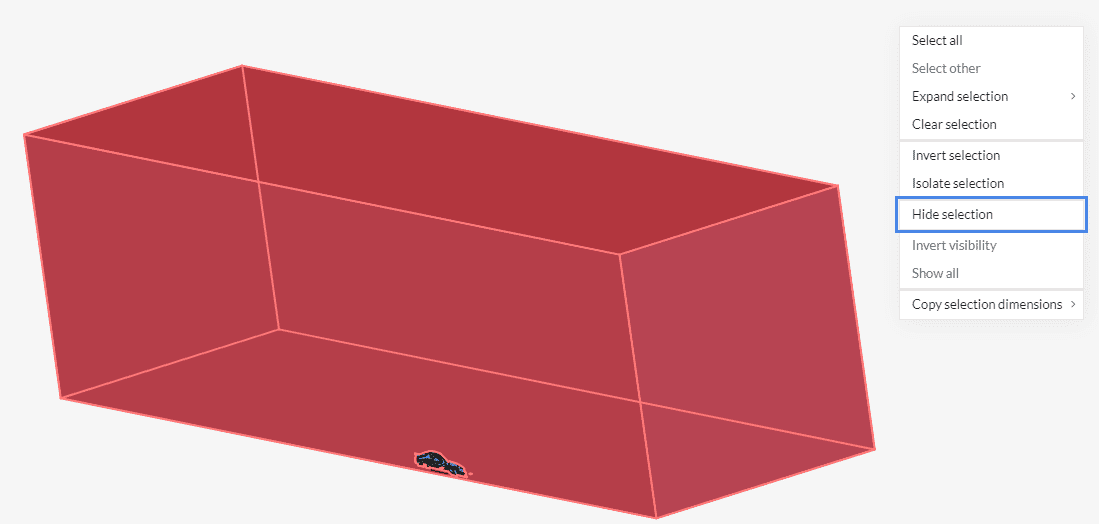
Let’s create three saved selections for this tutorial. To begin with, hide the walls of the flow region. To do this, select all six faces of the domain by rotating the model (they should turn to red). Then right-click in the viewer, and pick the ‘Hide selection‘ option, so they turn invisible.
After the walls of the domain are hidden, follow the steps below:
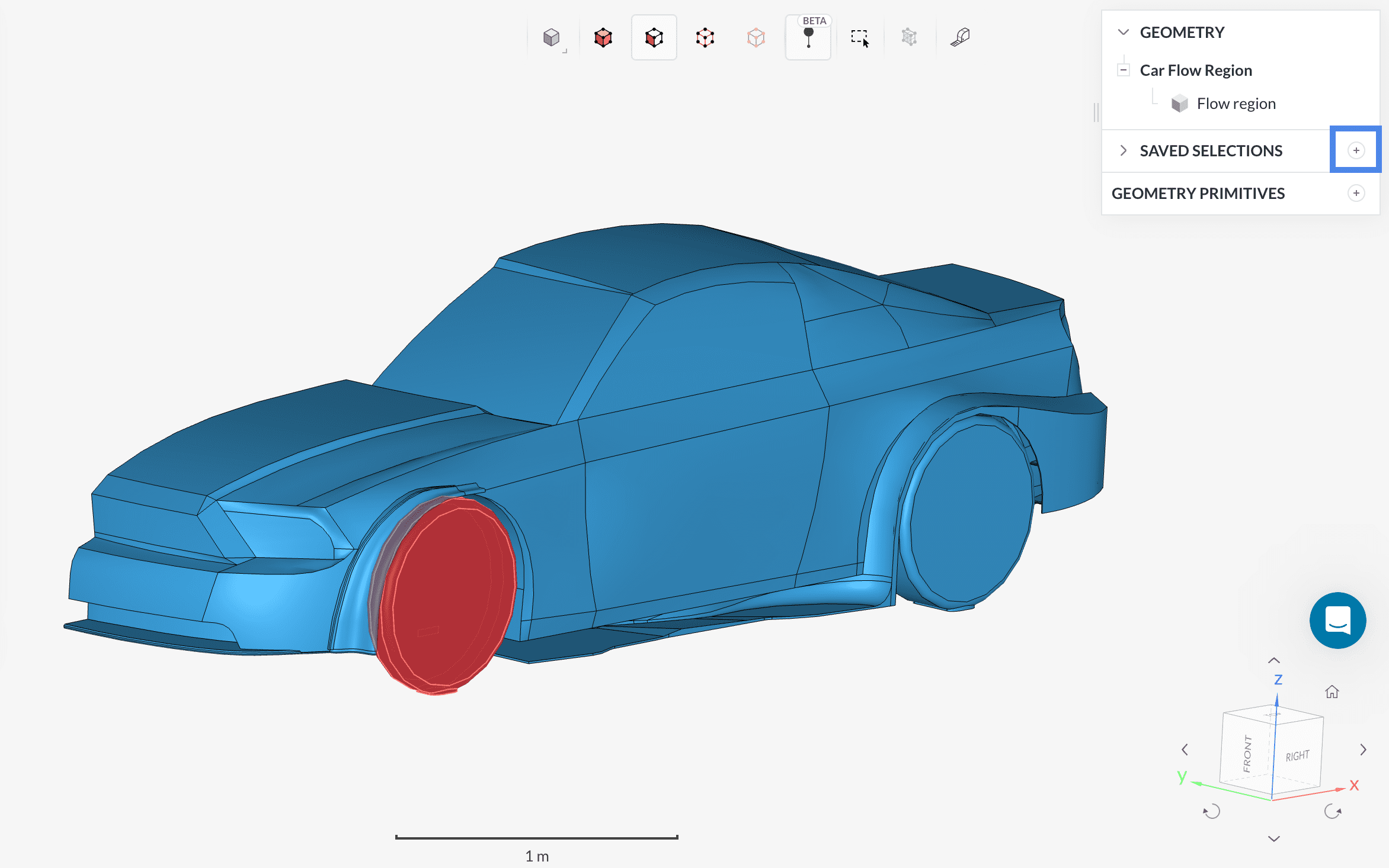
- Pick the 9 faces of the front wheel;
- Create a new set by clicking the ‘+ button ‘ next to the Saved Selections;
- Name the set appropriately (e.g., ‘Front Wheel’) and click on ‘Create New Set‘ after you are done.
- Repeat the same process for the 9 faces of the rear wheel.
Now, let’s create one saved selection for the remaining faces of the vehicle. Follow the steps below:
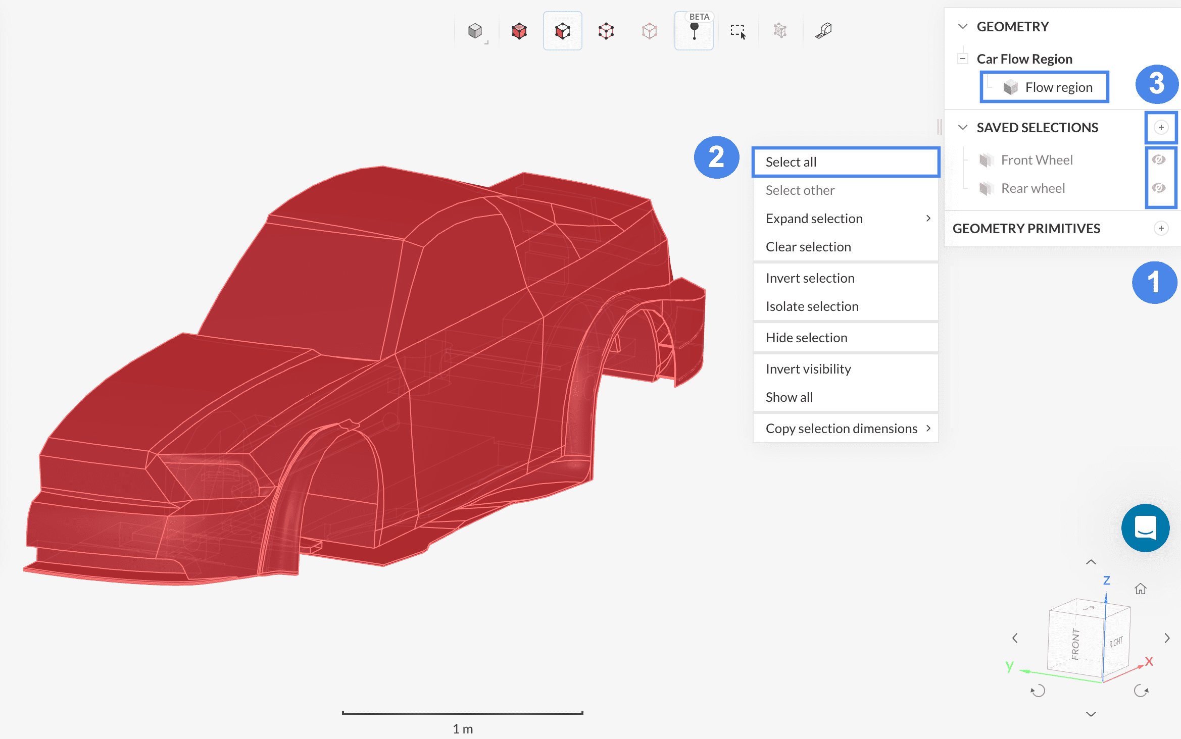
- Hide the front wheel and rear wheel saved selections by clicking on the eye icon next to them;
- Right-click in the viewer and click on ‘Select all ‘;
- Click on the ‘+ button ‘ next to Saved Selections;
- Name the newly created set appropriately (e.g., ‘Body’).
After creating the Body saved selection, you can make the walls reappear by right-clicking in the viewer and selecting ‘Show all’. The walls of the flow region will be necessary to assign boundary conditions later on in the tutorial.
2. Assigning the Material and Boundary Conditions
Now we are ready to set up the physics of the simulation.
2.1 Define a Material
In the simulation tree, click on the ‘+ button’ next to Materials.
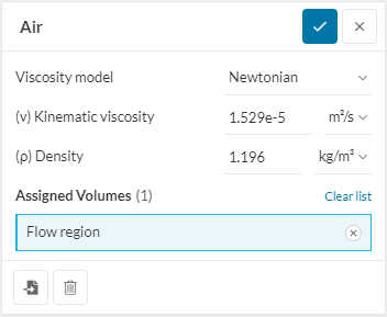
After opening the materials section, select ‘Air’ from the SimScale materials library. Click on ‘Apply’ to confirm your selection.
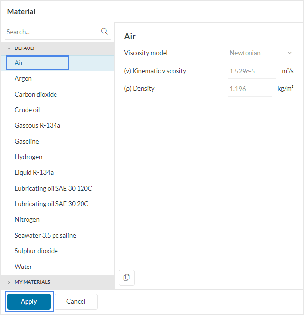
The flow region that was created at the beginning of the simulation setup is automatically assigned to the material:
Did you know?
For this tutorial, we will use the default values for the air properties. It’s possible, however, to edit each one of the values from Figure 19 by clicking on them.
2.2 Assign the Boundary Conditions
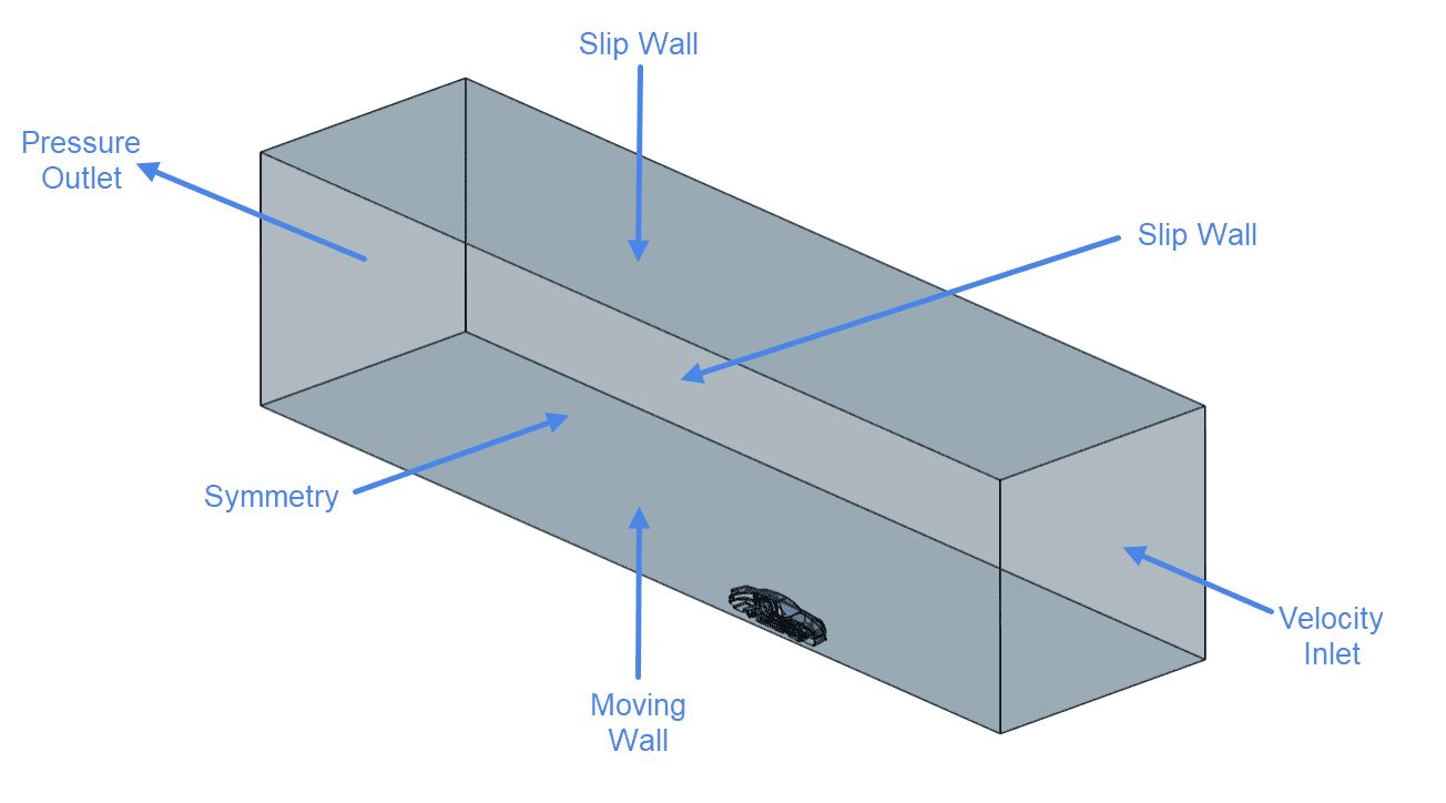
The physical situation simulated is a car moving with 20 \(m/s\). Now it is rather difficult to directly model the car’s velocity in a CFD simulation. We get the same result if we turn the situation around. Instead of a moving car and the still-standing street, we make the car stand still and let the air around the car and the street move with 20 \(m/s\).
An overview of the boundary conditions for the domain can be seen below:
Similarly, for the car wheels, the following boundary conditions are applied:
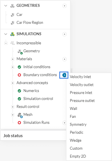
To create a boundary condition, click on the ‘+ button’ next to Boundary conditions, and select the desired type from the drop-down menu.
a. Velocity Inlet
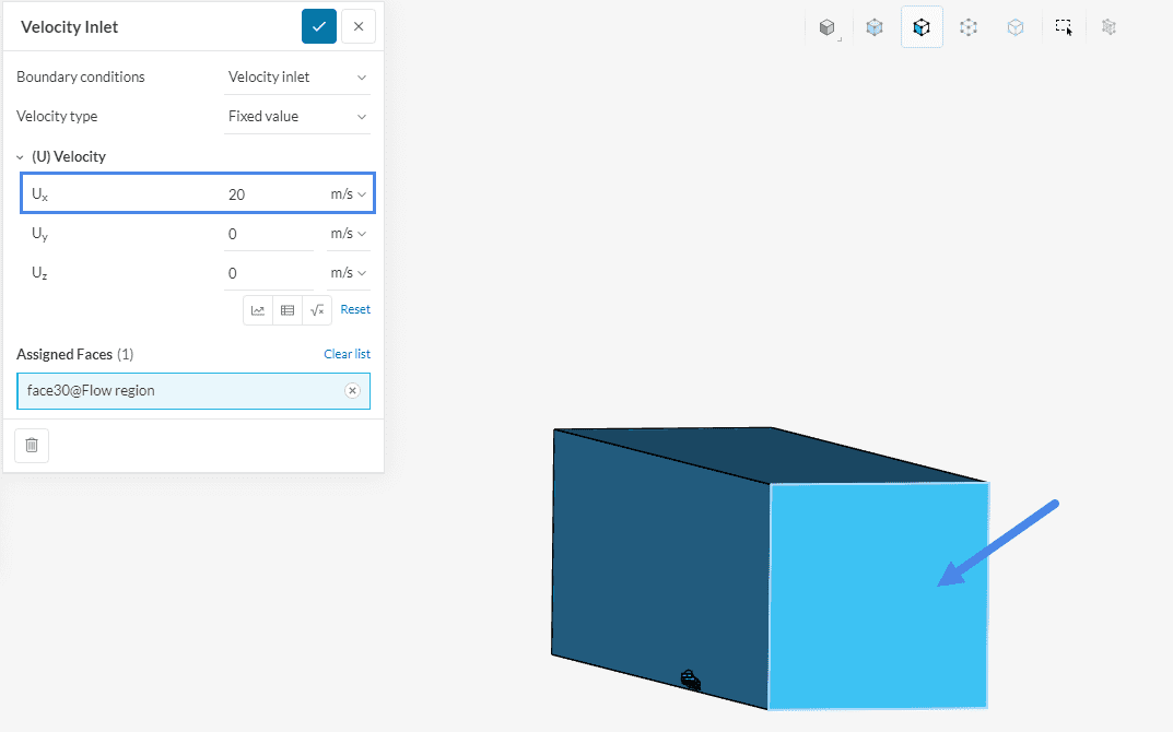
Let’s define the air velocity at the inlet face. To do so, create a new boundary condition, selecting ‘Velocity Inlet’ from the drop-down menu, as seen in Figure 22.
With a Fixed value velocity inlet boundary condition, the velocity that we define is a vector. You can use the orientation cube in the bottom-right corner of the viewer for reference. In this tutorial, set the velocity in the x-direction to ’20’ \(m/s\). Last assign the front face of the flow region to the boundary condition.
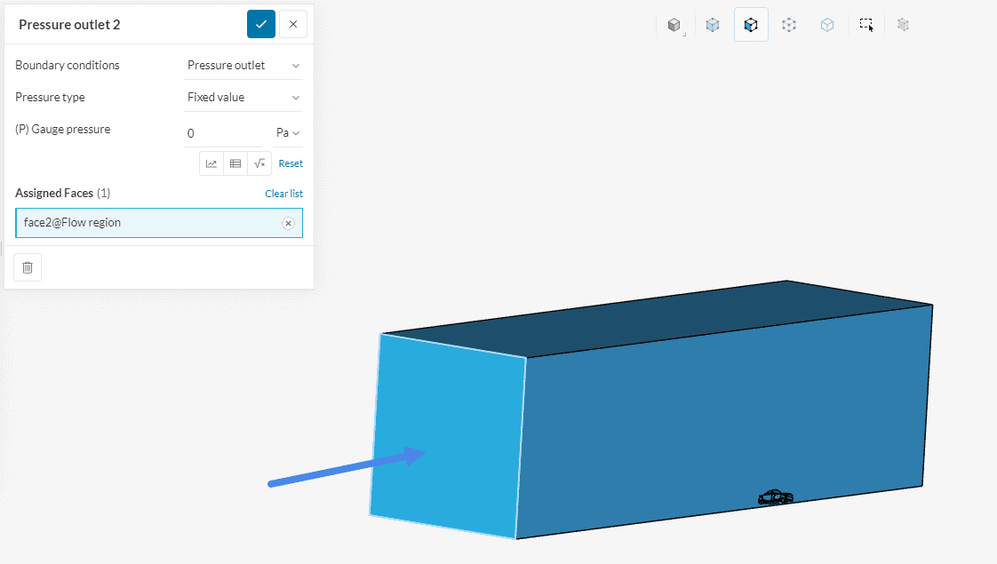
b. Pressure Outlet
We want to specify the outlet of the flow region as normal atmosphere, zero gauge pressure. Create a second boundary condition, this time a ‘Pressure Outlet’ and specify a fixed gauge pressure. The gauge pressure is relative to a reference value (ambient pressure, for example). Therefore, a pressure outlet condition with ‘0’ \(Pa\) gauge pressure is applied to the outlet face of the domain. Assign the back face of the flow region to this boundary condition.
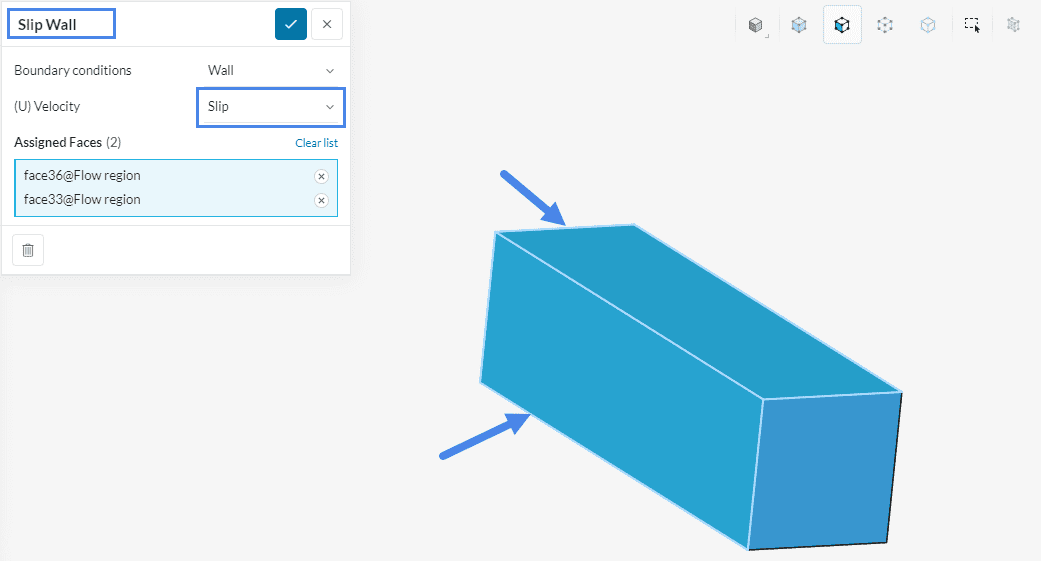
c. Walls: Slip Condition
For the third boundary condition, select ‘Wall’ from the drop-down menu. Set (U) Velocity to ‘Slip’.
The slip condition allows flow tangent to the face without the creation of a boundary layer, but won’t allow flow in a normal direction. This is a good approximation for the top and side faces of the flow region, which are far away from the car. Therefore, assign the slip wall condition to the top (XY-plane) and the right side (XZ-plane) of the domain, as seen below. Assign both, the right and the top face of the flow region to this boundary condition.
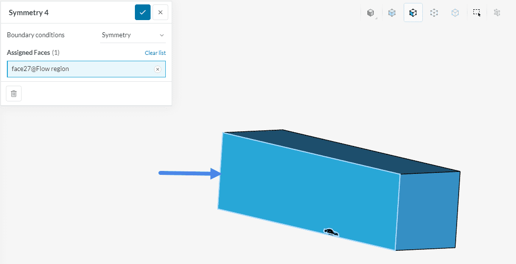
d. Symmetry
As previously discussed, a ‘Symmetry’ boundary condition will be applied to the symmetry plane, since we expect mirrored aerodynamic flow patterns on the two sides of the car. Assign the symmetry face to the boundary condition.
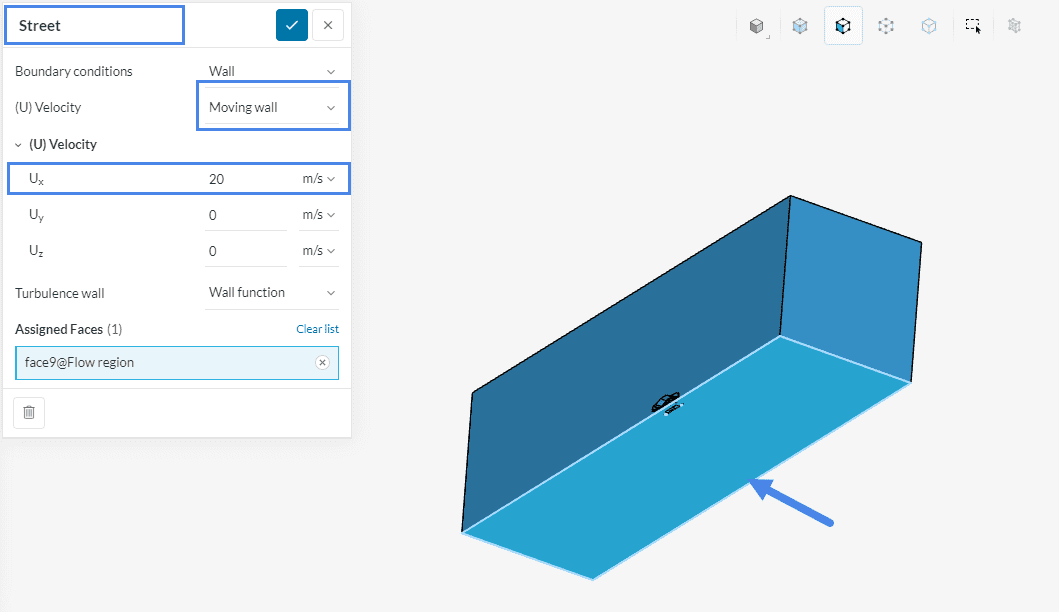
e. Wall: Moving Wall
Now, assign a boundary condition to the ground face which is the street. Create another ‘Wall’ boundary condition. For better clarity rename the boundary condition to ‘Street’. This time, set (U) Velocity to ‘Moving wall’. In this configuration, specify the tangential component for the fluid velocity on the assigned face.
Define a velocity of ’20’ \(m/s\) in the x-direction, which is the same vector that was defined for the velocity inlet boundary condition.
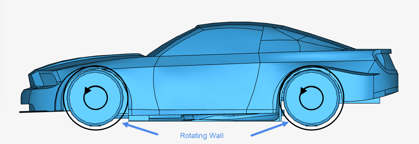
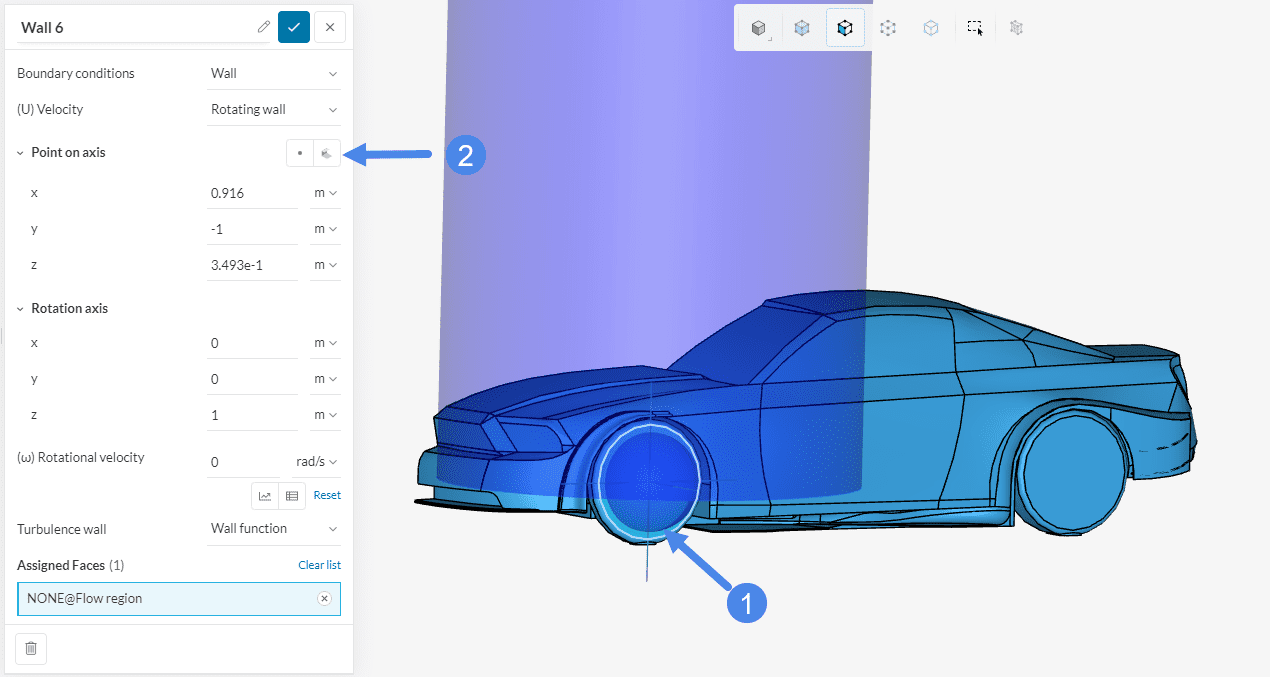
h. Wall: Rotating Wall – Front Wheel
We can model the rotating car wheels with a ‘Wall’ boundary condition. This time, select ‘Rotating wall’ for (U) Velocity. The following information is necessary to set up a rotating wall condition:
- Point on axis: The user should define a point on the axis of rotation. In our case, the center of the wheel should be used as a reference. In Figure 28, this can be done by selecting the center face of the wheel and selecting the ‘Pick center from current selection’ icon. This will automatically enter the center point of the face as the Point on axis.
- Rotation axis: This is the axis about which the faces will rotate. The direction of the rotation is given by the right-hand rule. In the right-hand rule, the thumb represents the rotation axis and the movement of the other fingers represents the direction of rotation. See Figure 29:
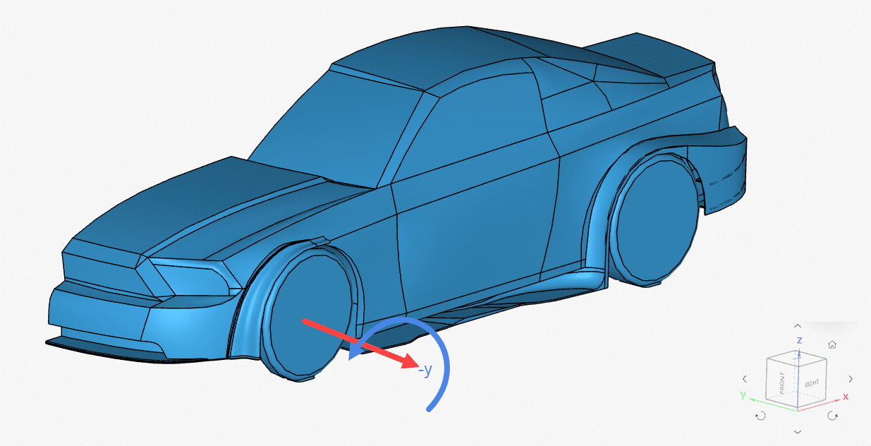
- (ω) Rotational velocity: The last parameter to define is the rotational velocity \(\omega\) (\(rad/s\)) for the wheels. It can be calculated using formula (1) below:
$$\omega = \frac {U} {r} \tag{1}$$
Where \(U \ [m/s]\) is the linear velocity of the car and \(r\ [m]\) is the radius of the wheel.
In our case, the car velocity is 20 \(m/s\) and the wheel radius is 0.3495 \(m\). Therefore, our rotational velocity \(\omega\) is ‘57.22’ \(rad/s\).
Now we have the necessary information to set up the rotating wall condition for the front wheel, as seen in Figure 30 below:
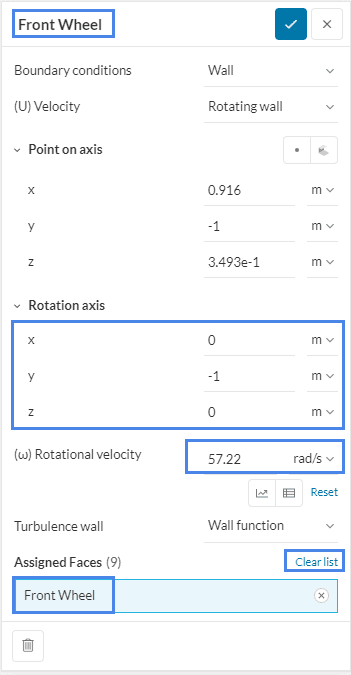
- Rename the boundary condition to ‘Front Wheel’
- Define (U) Velocity as a ‘Rotating wall’;
- Specify ‘-1’ in the y-direction for the Rotation axis. The Rotational velocity is ‘57.22’ \(rad/s\).
- Lastly, clear the list of assigned faces and assign this boundary condition to the previously defined ‘Front Wheel’ saved selection.
Simulating Rims
In this tutorial the rims of the car are simplified with a closed face. This is a simplification to most street vehicles. The rim of a wheel is usually made of spokes, which allows air to pass through the rim. In order to capture the effects of a rotating rim the advanced concept of a rotating zone can be used.
You can learn more about this concept on this documentation page.
g. Wall: Rotating Wall – Rear Wheel
The same procedure is also followed for the rear wheel. The only difference between the front wheel and the rear wheel boundary conditions will be the Point on axis coordinates.
Please set up the final wall boundary condition as shown below:
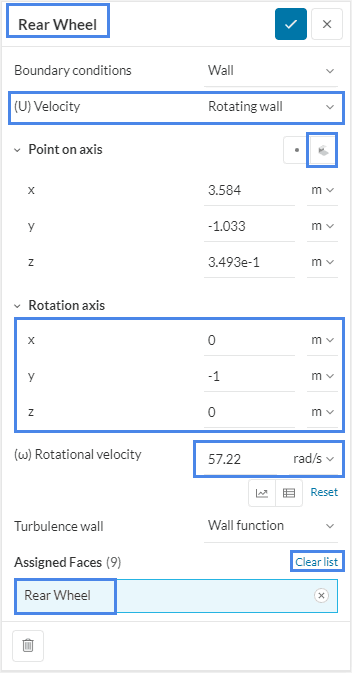
- Rename the boundary condition to ‘Rear Wheel’
- Define (U) Velocity as a ‘Rotating wall’;
- Select the Point on axis using the same method as for the Front Wheel boundary condition.
- Specify ‘-1’ in the y-direction for the Rotation axis. The Rotational velocity is ‘57.22’ \(rad/s\).
- Lastly, assign this boundary condition to the previously defined ‘Rear Wheel’ saved selection.
Automatic boundary condition assignment
For all faces not assigned to a specific boundary condition SimScale will set the boundary to a no-Slip wall condition. In this tutorial the car body minus the wheel is automatically treated as a no-slip wall boundary.
Find in this article relevant information about wall functions and other wall treatments.
2.3. Simulation Control
In the simulation tree, click on the ‘Simulation control’ tab, and configure it as shown:
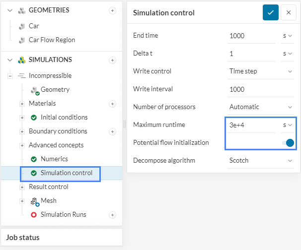
- Change the Maximum runtime for the simulation to ‘30000’ seconds;
- ‘Enable’ Potential flow initialization. This setting initializes the velocity field and enhances stability in the early iterations.
Did you know?
In a steady-state simulation, the End time and Delta t parameters control the number of iterations to be performed. With the default settings, a simulation consists of a total of 1000 iterations, which is enough for most simulations to converge.
For more notes on the simulation control settings, please visit the following page: Simulation control for fluid flow simulations.
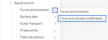
2.4 Results Control
Lift and drag coefficients are some of the most important parameters when evaluating the performance of the flow aerodynamics of a vehicle. Therefore, let’s create a ‘Force and moment coefficients’ result control, as shown below:
Please set up the result control as below:
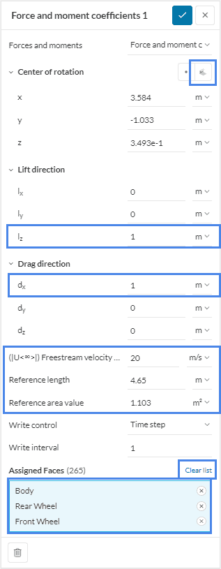
- The Center of rotation coordinates of our car is determined as follows:
- Use the center of the Rear Wheel for Center of rotation. The coordinates can be obtained using the same pick center from current selection option as used for the rear wheel boundary condition.
- Set the positive z-axis as the Lift direction by entering ‘1’. The other axes receive a value of ‘0’;
- Set the positive x-axis as the Drag direction by entering ‘1’. The other axes receive a value of ‘0’;
- Apply ’20’ \(m/s\) as (|U<∞>|) Freestream velocity magnitude, which is the same magnitude that was defined for the velocity inlet boundary condition;
- The Reference length is the car’s length along the x-axis. Our car’s length is ‘4.65’ \(m\);
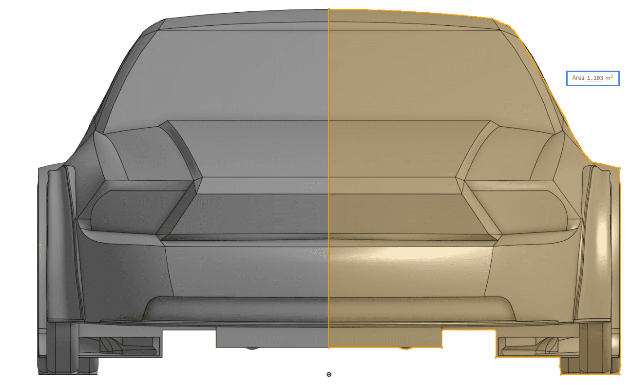
- The Reference area value is a projection of the frontal car area onto a plane. It’s important to note that, as we’re using half of the car geometry, the area projection must account only for half of the model.
- Clear the list of assigned faces and assign the result control to all of the car faces. The easiest way to do that is by assigning the three previously created saved selections.
Aerodynamic Balance
When setting up the force coefficient report the center of the rear wheel is selected. This setup helps to calculate the aerodynamic balance of the car, Dividing the result of the moment report with the wheelbase the force coefficient of the front axle is calculated. Dividing the force coefficient of the front axle with the total lift coefficient results in the aerodynamic balance in the percentage of the frontal load. $$ \%_{Front} = \frac{Coef.Moment_{Rear}*Reference\ Length}{Wheelbase * Coef. Lift_{Total}} $$
Important
Be careful when setting up the result control parameters, as they are used by the algorithm to calculate the drag and lift coefficients.
For the drag and lift formulas, and more examples on how to set up the forces and moment coefficients result control, please refer to the following articles:
How to analyze the pitch, lift, and drag coefficients?
Why are my lift and drag coefficients too big/small?
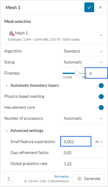
3. Mesh
For the meshing operation, we recommend using the standard algorithm. The standard meshing algorithm is a good choice in general, as it is quite automated and delivers good results for most geometries, with the following default properties, including a Small feature suppression of ‘0.001’ \(m\) under the Advanced settings:
Did you know?
Often, large changes in the mesh’s cell sizes only occur in few regions. Increasing the global mesh refinements increases the number of cells drastically.
When using the standard mesher, SimScale offers a physics-based meshing option, which automatically refines the regions around the inlets and outlets.
You can also do this manually, by using one of the local refinement options, foremost being surface sizing and Volume sizing refinements.
If you want to learn more about the Standard meshing algorithm, please have a look at the relevant documentation page.
3.1 Adding Refinements
Why do we need mesh refinements?
In external aerodynamic simulations, as air flows around the body, two regions have important physical effects: the regions close to the car body and the wake region, which develops downstream from the object.
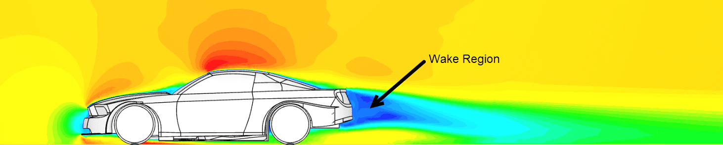
Since the gradients in velocity and pressure are large in those areas, they require finer cells to be resolved accurately. Therefore, further refinements will be necessary.
Use refinements to more accurately capture the wake and the aerodynamic flow around the car. A volume custom sizing is used to refine the volume mesh for one or more user-specified geometry primitives.
To add a volume custom sizing to your mesh, first, create two geometry primitive boxes. On the right-hand panel click the ‘+ button’ next to the geometry primitives and select the cartesian box.
a. Volume Custom Sizing
Set the values for the first volume (Far Field) as seen below.
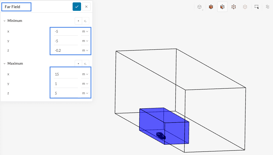
Rename the first box ‘Far Field’ and add the dimensions as follows:
- Minimum (x) value: ‘-5’ \(m\)
- Minimum (y) value: ‘-5’ \(m\)
- Minimum (z) value: ‘-0.2’ \(m\)
- Maximum (x) value: ’15’ \(m\)
- Maximum (y) value: ‘1’ \(m\)
- Maximum (z) value: ‘5’ \(m\)
Repeat the process to create the second smaller box. This box is used to even further refine the mesh directly around the car.
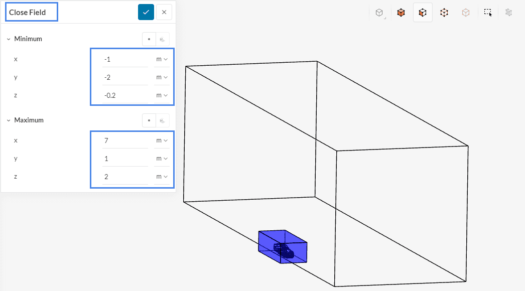
Rename the box to ‘Close Field’ and the dimensions of the box are as follows:
- Minimum (x) value: ‘-1’ \(m\)
- Minimum (y) value: ‘-2’ \(m\)
- Minimum (z) value: ‘-0.2’ \(m\)
- Maximum (x) value: ‘7’ \(m\)
- Maximum (y) value: ‘1’ \(m\)
- Maximum (z) value: ‘2’ \(m\)
Notice how the boxes extend further downstream from the car. The objective is to capture the high gradients from the wake, which is pictured in Figure 37.
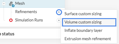
Next, create a new Volume custom sizing by clicking on the ‘+ button’ and selecting ‘Volume custom sizing’.
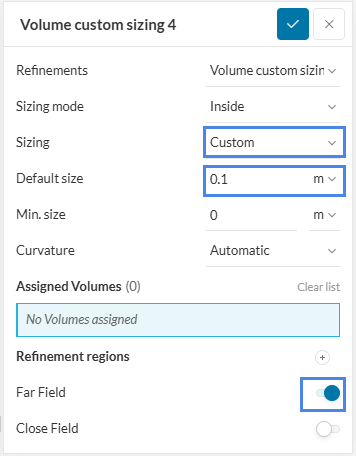
You can rename the volume custom sizing to ‘Volume Custom Sizing Far Field’, for example, if needed. Set Sizing to Custom the Default size to ‘0.1’ \(m\) and toggle on the Far Field selection:
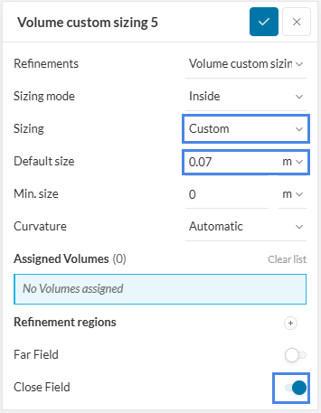
Repeat the process for the Close Field. As the smaller box is closer to the surface, a finer discretization will be enforced. Please set the Default size to ‘0.07’ \(m\):
b. Surface Custom Sizing
To refine the cells directly at the wheel faces a surface custom sizing refinement is used. This refinement is applied to faces and limits the cell edge lengths based on the input.
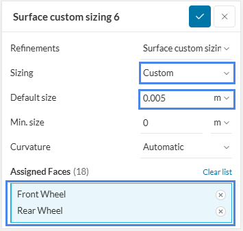
Create a ‘Surface custom sizing’ refinement and set the Sizing to Custom and Default size to ‘0.005’ \(m\). Assign it to both ‘Front Wheel’ and ‘Rear Wheel’ saved selections, to capture the region next to the rotating walls accurately.
3.2 Meshing Results
Now you can go back to the main meshing settings and click on ‘Generate’, as in Figure 36. Note that this is not a mandatory step: You can also just start the aerodynamic flow simulation and the mesh will be created automatically. However, let’s have a look at the finished mesh in this simulation before starting the simulation.
This mesh will take around 15 to 20 minutes to complete and this is what it will look like:
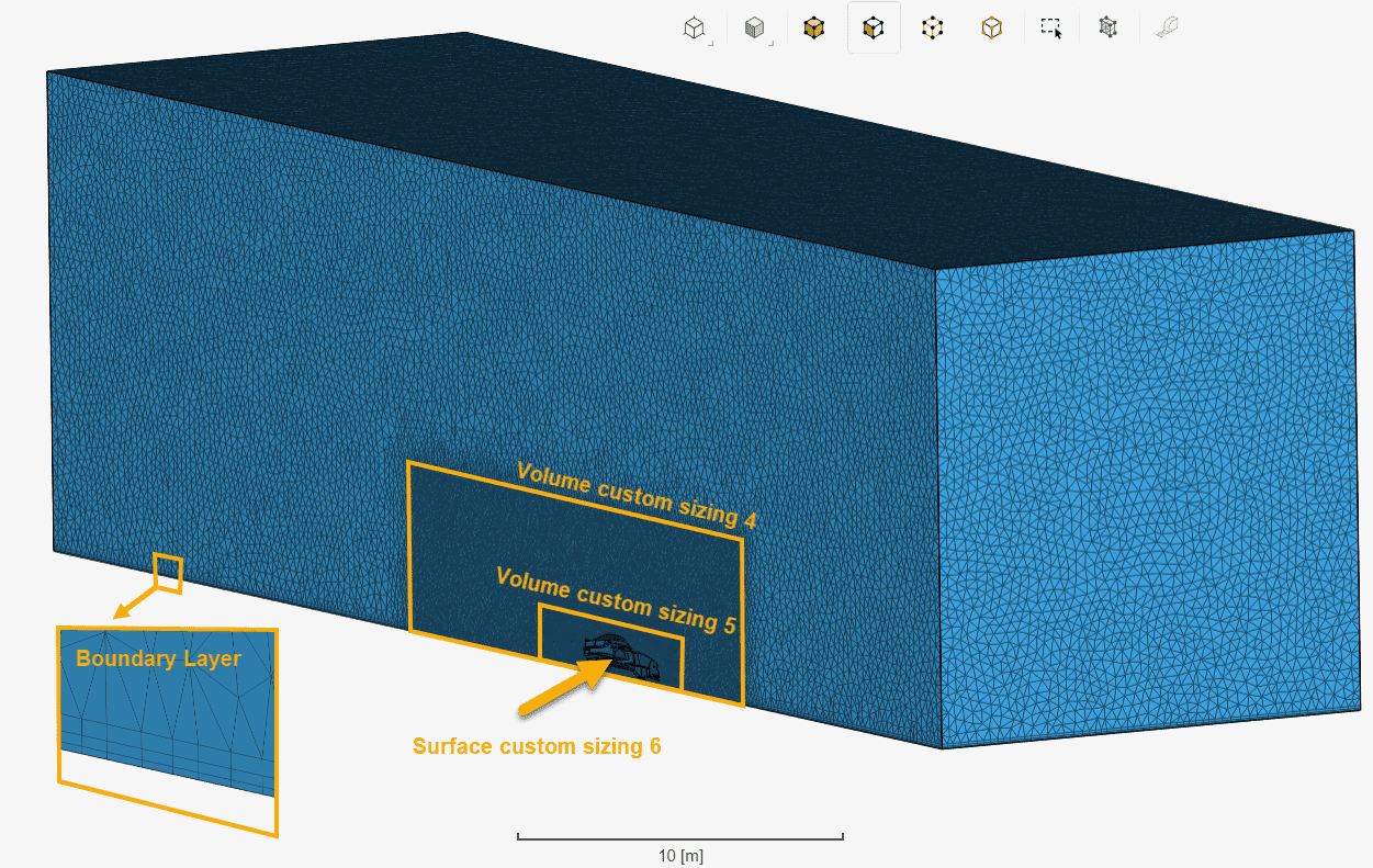
Be Aware
This tutorial presents how the simulation is set up for a successful CFD run. The setup for this tutorial is simplified. To ensure the reliability of the results, a series of studies have to be performed.
Further tests with finer meshes, improved layering control, extended flow region, etc., should be performed.
Naturally, it’s important to make sure that each of the simulation runs are also converging. For bigger meshes, it might be necessary to prescribe more iterations.
For more insights on how to assess convergence in a CFD simulation, please refer to this documentation page.
4. Start the Simulation
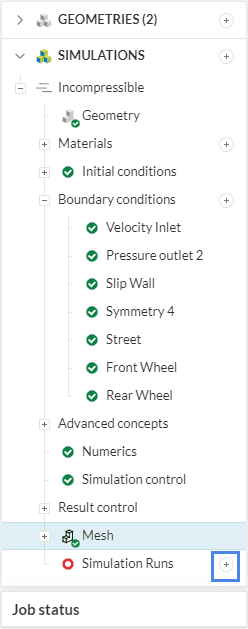
The simulation setup is now ready. We can proceed to create a new simulation run. To do so, click on the ‘+ button’ next to Simulation Runs.
This way, if not generated in advance, the mesh will be generated, and, afterward, the simulation run will start automatically. While the simulation results are being calculated, you can already have a look at the intermediate aerodynamic flow results in the post-processor. They are being updated in real-time!
You will also find a link to the finished project at the end of the tutorial.
Note
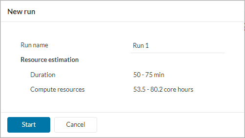
A red warning message may appear, stating that the duration of the simulation exceeds the maximum runtime. The defined maximum runtime of 30000 seconds will be enough for this simulation, therefore, please proceed by clicking on ‘Start’:
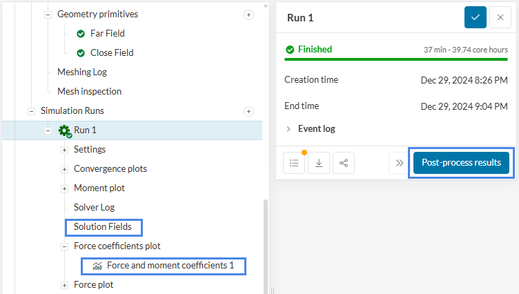
The simulation run takes about 35 to 40 minutes to finish. At this point, you can access the post-processing environment by clicking on ‘Solution Fields’ or ‘Post-process results’. You can also check the ‘Force and moment coefficients 1’ graphs under result control.
Note
With these particular mesh settings, the ‘Event log’ also returns a warning that it has defeatured a few faces that were added to result control. These are very small or narrow faces in the CAD that get defeatured because of the mesh settings being relatively coarse. Therefore, you can safely ignore this message in this case, but two possible alternatives here are a finer mesh around the car to be able to resolve these faces or a cleaner CAD model in the first place.
5. Post-Processing
5.1 Force and Moment Coefficients
The drag and lift coefficients are available in the ‘Force and moment coefficients’ tab:
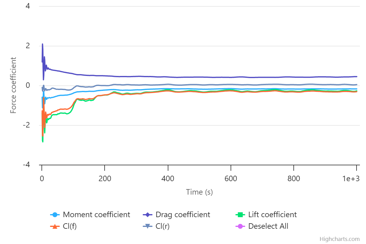
The plot shows you how the coefficients are changing throughout the simulation process, as the iterations go on. In a converged simulation, the coefficients will stabilize around a value.
Therefore, in a steady-state simulation, the intermediate results are important to assess convergence. The final, converged solution is the one that should be analyzed to obtain the aerodynamic flow parameters.
Calculating the Aerodynamic Balance
From the force and moment coefficient report it can be seen that a moment coefficient of -0.18 and a lift coefficient of -0.27 is calculated. As the force and moment coefficient report was defined at the center of the rear wheel the aerodynamic balance of the car can be calculated using the formula \(1\) below.
$$\%_{Front} = \frac{Coef.Moment_{Rear}*Reference Length}{Wheelbase *Coef.Lift}\tag{1}$$
The wheelbase of the car is 2.665 \(m\) and the reference length was set to 4.6 \(m\). Using these values an aerodynamic balance of 115% front is calculated. This means that most of the aerodynamic force is on the front axle of the car.
5.2 Surface Visualization
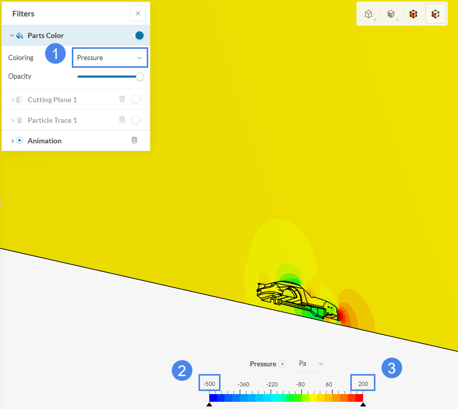
After accessing the post-processor, you can use several post-processing filters to further analyze the results. If the pressure distribution is not yet visualized, go to Parts color and change the Coloring to ‘Pressure’. The legend at the bottom of the page includes a default range set by the lowest and highest values inside the domain. By clicking on the upper and lower limits and editing their values, you can control the quality of visualization, making sure that the color map on the surface is insightful.
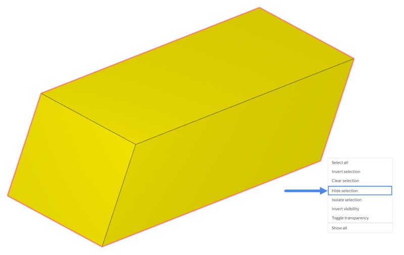
To better visualize the aerodynamic flow around the car you can hide the flow region by selecting all faces of the flow region, right-clicking your mouse, and choosing ‘Hide selection’.
In Figure 52, we have the pressure contours on the car body. As previously discussed, these are gauge pressures. In the areas where aerodynamic flow stagnation occurs (e.g., on the bumper), pressure exhibits larger values. To add a smooth distribution of the colors on the vehicle, right-click on the legend at the bottom, and select ‘Use continuous scale’ :
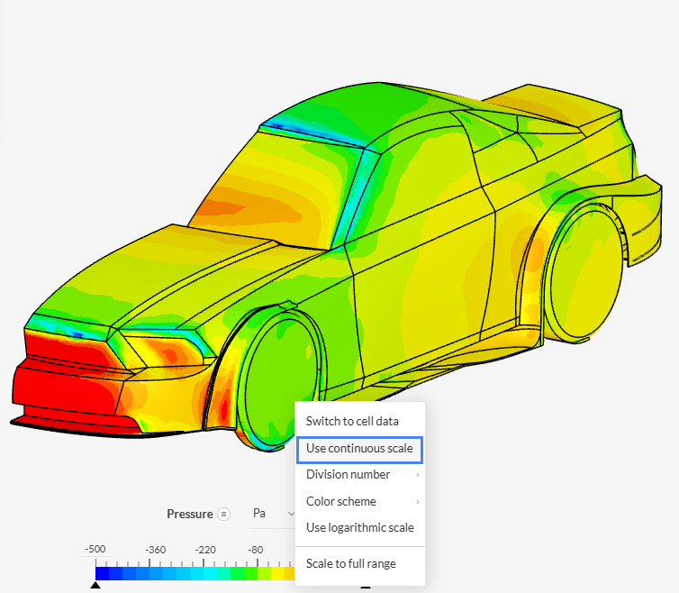
The upgrade in the visualization quality is evident:
5.3 Cutting Planes
If you want to observe the aerodynamic flow characteristics around the car, then you can obtain some insights with a ‘Cutting Plane’:
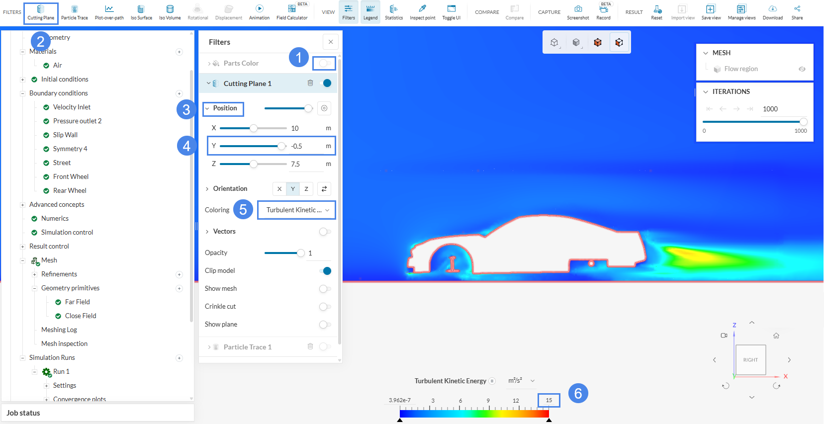
Configure the cutting plane by following the steps below:
- Change the Position by changing the Y coordinate to: ‘-0.5’;
- Make sure the Orientation is on the ‘Y’ axis;
- Change the Coloring to ‘Turbulent Kinetic Energy’;
- Set the maximum value of the range to ’15’ \(\frac{m^2} {s^2}\).
From the figure above, we can see that the car creates a disturbance in the aerodynamic flow which produces high turbulent kinetic energy, especially behind the trunk, closer to the ground.
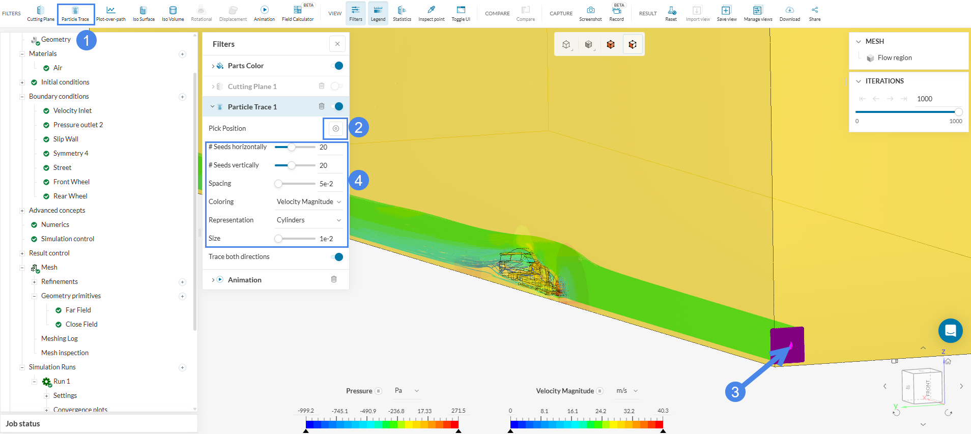
5.4 Streamlines and Animation
Streamlines are useful to visualize the aerodynamic flow path around the car. To do this, select ‘Particle Trace’ from the Filters panel and its settings will be shown.
Next, pick the start position of the particles by clicking the button beside Position.
- Place this at the inlet of the flow region and the streamlines will be shown from the start point;
- Modify the number of particles under # Seeds horizontally and # Seeds vertically. Use ’20’ points horizontally and ’20’ points vertically.
- Change the Spacing of the streamlines to ‘5e-2’ and the size to ‘1e-2’;
- The Trace both directions option is not necessary here, you can disable it;
- Set the range of the velocity magnitude scale to ‘[0, 25]’ \(m \over s \).
Animations can be started by choosing ‘Animation’ from the Filters panel. After changing the Animation type to ‘Particle Trace’, click the ![]() play button to start the animation.
play button to start the animation.
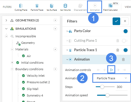
The result is shown in the animation below, for better visualization the traces has been changed from cylinders to comets:
When combining the pressure distribution on the surfaces of the car with the velocity streamlines around the car, we can see that high pressure is created at the front when the velocity is at the lowest. Aerodynamic flow seems to be accelerating as it travels over the roof and beyond. A Suction region with very low velocities can be analyzed with blue streamlines.
You can analyze the aerodynamic flow results further with the SimScale post-processor. Have a look at our post-processing guide to learn how to use it.
Congratulations! You finished the aerodynamic flow behavior tutorial!
Note
If you have questions or suggestions, please reach out either via the forum or contact us directly.
Last updated: April 4th, 2026
Did this article solve your issue?
How can we do better?
We appreciate and value your feedback.


