What Is a Surrogate Model?

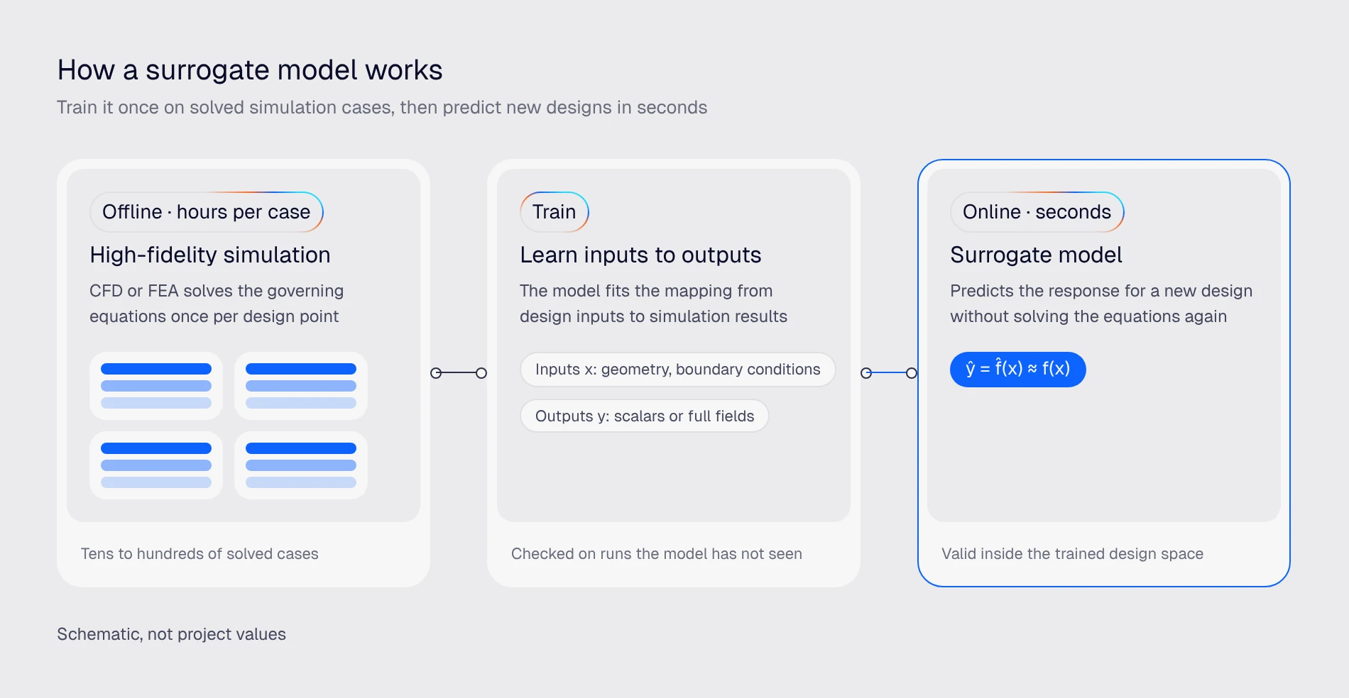
A surrogate model is a fast approximation of an expensive simulation. It’s trained on the inputs and outputs of solved cases, then predicts the result for a new design in seconds instead of hours.

Engineers reach for one when a single CFD or FEA run takes hours and the design question needs hundreds of answers. At Convion, a solver-driven optimization of one ejector “easily takes weeks,” in the words of its thermofluids lead. With a trained surrogate in the loop, the same optimization ran in minutes.

Surrogate model definition

A surrogate model (also called a metamodel, response surface model or emulator) approximates the input-output behavior of a high-fidelity simulation. It’s trained on a set of solved simulation cases and predicts the response for new inputs without solving the governing equations again.

$$ \hat{y} = \hat{f}(\mathbf{x}) \approx f(\mathbf{x}) \tag{1} $$

Here \(\mathbf{x}\) is the vector of design inputs (geometry parameters, boundary conditions, operating points), \(f\) is the simulation and \(\hat{f}\) is the surrogate, trained on \(N\) solved samples \((\mathbf{x}_i, f(\mathbf{x}_i))\).

The output can be a few scalars, such as pressure drop, drag coefficient or peak temperature. It can also be a full field, such as pressure and velocity on every surface of the part. Field surrogates are what most engineers mean by an AI surrogate model for CFD.

Surrogate model vs physics solver

A physics solver computes each case from first principles. A surrogate model learns from cases the solver has already computed. That difference sets where each one belongs.

Criterion	Physics solver (CFD, FEA)	Surrogate model
How it gets the answer	Solves the governing equations on a mesh	Maps inputs to outputs learned from solved cases
Time per new design	Minutes to hours	Milliseconds to seconds
Up-front cost	Setup and meshing per case	Tens to hundreds of solver runs, plus training
Valid range	Any case the physics models cover	Only inside the design space it was trained on
Accuracy depends on	Mesh, physics models, numerics	Quality and coverage of the training data
Best for	New physics, one-off cases, final validation	Design space exploration, optimization, sensitivity studies, real-time use

In practice the two work together. The surrogate screens thousands of variants, and the solver confirms the shortlist. For more on that hybrid pattern, see AI simulation explained.

Types of surrogate models

Pick the type by the number of inputs, the number of solver runs you can afford and whether you need scalars or full fields [1].

Type	How it works	Fits when
Polynomial response surface	Fits a low-order polynomial by least squares	Few inputs, smooth response, small run budget
Kriging / Gaussian process	Interpolates between samples using their spatial correlation; returns an uncertainty estimate	Expensive runs, tens to low hundreds of samples, you need error bars
Radial basis functions	Sums distance-weighted basis functions centered on the samples	Scattered samples, moderate number of inputs
Polynomial chaos expansion	Expands the output in orthogonal polynomials of random inputs	Uncertainty quantification
Neural networks	Learns a layered nonlinear mapping from data	Many inputs, strongly nonlinear physics, full 3D field outputs, larger data sets

The classic methods fit smooth, low-dimensional problems well. They struggle when the physics turns sharply nonlinear. Convion learned this firsthand: its earlier attempts with traditional surrogate modeling “proved insufficient to capture the extreme non-linear behavior present in this regime,” so the team moved to neural network models trained on 3D CFD (Convion case study).

Surrogate models, reduced-order models and physics-informed machine learning

These three terms overlap in search results, but they build the fast model in different ways.

Approach	How it’s built	What it needs	Trade-off
Surrogate model (data-driven)	Learns from solver outputs; treats the solver as a black box	Solved cases from any solver	Simple to build from existing runs; valid only inside the training range
Reduced-order model (ROM)	Projects the governing equations onto a small set of dominant modes, for example by proper orthogonal decomposition (POD) [4]	Solution snapshots plus access to the equations or operators	Keeps more of the physics; harder to build around commercial solvers
Physics-informed machine learning (for example PINNs)	Trains a neural network whose loss penalizes violations of the governing equations [3]	The equations, with little or no solver data	Physics built into training; training is often slow for complex 3D flows

The boundaries are blurring. Many current AI surrogates for CFD learn from solver data and add physics constraints during training, which is why the press often calls them physics-informed.

How surrogate models are trained

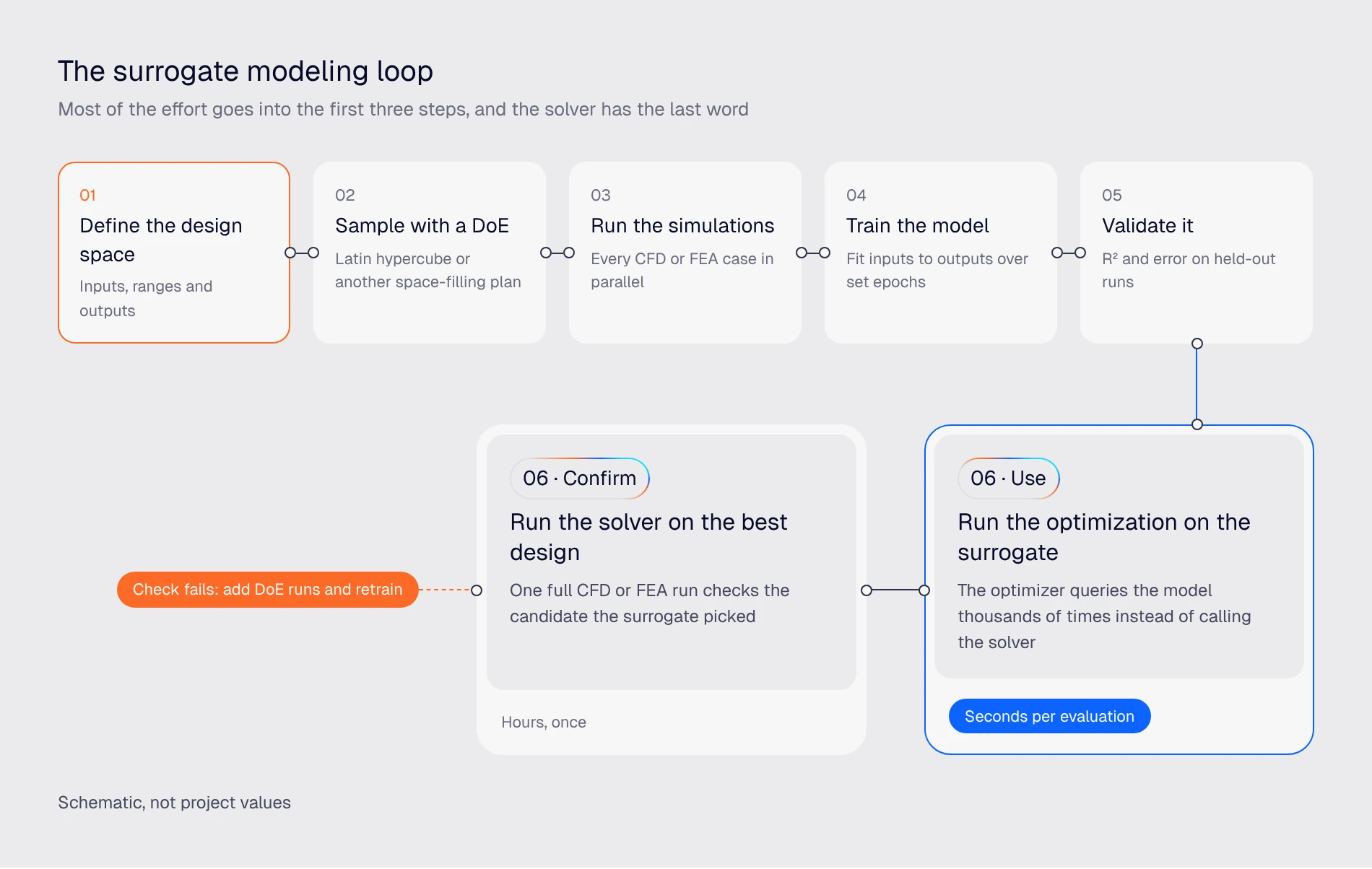
Training a surrogate is a six-step loop. Most of the effort goes into the first three.

1. Define the design space. Choose the input parameters, their ranges and the outputs you care about.
2. Sample it with a design of experiments. A space-filling plan such as Latin hypercube sampling [6] spreads the runs across every input at once. See design of experiments in engineering for the methods.
3. Run the simulations. Each sample is a full CFD or FEA case. Running them in parallel turns weeks of sequential solving into hours.
4. Train the model on the solved cases.
5. Validate it on runs the model hasn’t seen.
6. Use it, then confirm. Run the optimizer or design study against the surrogate, then run the solver on the final candidate.

Design of experiments for training data

Training data comes from a DoE, which needs far fewer runs than a solver-driven optimization. An optimizer walks the design space step by step and can need thousands of evaluations. A DoE covers the space once, up front, in hundreds.

“When we’re training or doing CFD simulations for training a Physics AI, we’re not doing optimization,” said Armin Narimanzadeh, Thermofluids & Simulations team lead at Convion. “It’s a DoE problem, and you could do less with a DoE problem.”

Where the DoE starts matters too. Convion runs 0D and 1D calculations first to find the promising region, then spends its 3D CFD budget there.

How many simulations do you need?

There’s no universal number, but three reference points help.

• Rule of thumb: about 10 runs per input variable is a common starting point for Gaussian process surrogates [2].
• Minimum in SimScale: AI model training needs at least 20 simulation runs, and more data usually improves accuracy (AI model training docs).
• A real case: Convion trained separate models on 128, 256 and 512 CFD runs of an ejector. Going from 256 to 512 runs gained little. With a tight mesh around the nozzle, where the gas compresses, 128 runs were enough for this case.

The Convion test is the method to copy. Train on growing subsets of your data and stop adding runs when the validation error stops falling. Data quality in the regions that drive the result counts for more than raw run count.

Training and validating the model

Neural network surrogates train over a set number of epochs, one epoch being one pass through the training data. Too few and the model underfits. Too many and it memorizes the training runs and generalizes poorly. In SimScale you set the number of epochs and a target confidence score before training starts, then review how the model performed across the epochs before releasing it to your team.

Check these before you trust a surrogate:

• R² close to 1 on validation runs.
• Mean absolute error (MAE) and maximum mean absolute percentage error close to zero for each output quantity.
• Training loss vs validation loss. If validation loss is much higher, the model is overfitting. Retrain with more data or fewer epochs.
• A solver run on the final design. The last word belongs to the physics.

Surrogate-based optimization: the Convion example

Convion designs solid oxide fuel cell and electrolyzer systems. One component, an ejector that recovers high-temperature process gas, had coupled, competing performance targets and a highly nonlinear design space. Finding the best configuration with simulation-driven optimization “would have taken months,” according to Armin.

The team replaced the solver inside the optimization loop with a surrogate:

1. Generate data. A parametric CAD model in Onshape fed a DoE of hundreds of CFD runs, executed in parallel on SimScale.
2. Train. The results trained a Physics AI model. Models on 128, 256 and 512 runs showed where more data stopped helping.
3. Run the optimization. A genetic algorithm queried the model instead of the CFD solver. A full optimization now takes minutes, and a new optimized design takes under an hour.
4. Validate. Armin ran a full CFD-driven optimization alongside the first one. For this case, the model predicted performance within 5% of high-fidelity CFD.

The design that came out met every performance target in 50% less physical volume. And because the validated model is reusable, a new component for changed boundary conditions is now “half a day maximum away,” down from weeks.

Most surrogate-based optimizations are multi-objective, as Convion’s was. Querying a surrogate in milliseconds is what makes mapping a full Pareto front affordable.

When not to use a surrogate model

A surrogate is the wrong tool in these cases:

• The design falls outside the training range. Surrogates interpolate well and extrapolate badly. “You get the results that you’re trained for,” as Armin put it. Outside the DoE bounds, run the solver.
• The analysis is a one-off. If you need three runs, the training data costs more than the answer.
• The response jumps. Flow regime changes, buckling or contact switching create discontinuities that smooth surrogates blur unless you sample densely around them.
• The result is a sign-off. Certification and final design release need a solver result.

Surrogate modeling in SimScale

SimScale runs the whole loop in the browser. You can generate the DoE with parametric studies or have the Engineering AI agent set it up, run every case in parallel in the cloud, then train a model on the results. In a live demo at Agentic Unlocks, a drone model’s training job was submitted in about a minute and ready in about 40 minutes on cloud GPUs. The trained model then returned field predictions in seconds, shown side by side with the CFD result.

Because the surrogate and the solver share the same setup, you can switch from a prediction to a full CFD or FEA run of the same design in a few clicks.

FAQ

What is the difference between a surrogate model and a reduced-order model?

A surrogate model learns the input-output relationship from solved simulation cases and treats the solver as a black box. A reduced-order model projects the governing equations onto a small number of dominant modes, so it needs access to the equations or solver internals. Both give fast answers; the surrogate is simpler to build from existing runs.

How many simulations do I need to train a surrogate model?

A common starting point is about 10 runs per input variable for Gaussian process models, and SimScale’s AI model training needs at least 20 runs. Neural network surrogates that predict full 3D fields usually need hundreds. Convion found 256 runs gave nearly the same result as 512, and 128 were enough with a fine mesh in the critical region.

How accurate is an AI surrogate model compared to CFD?

Accuracy depends on the training data and on staying inside the trained design space, so check it on validation runs with metrics such as R² and mean absolute error. In Convion’s ejector case, the model predicted performance within 5% of high-fidelity CFD. Always confirm the final design with a solver run.

Is a surrogate model the same as a physics-informed neural network?

They’re different methods. A standard surrogate model learns only from simulation data. A physics-informed neural network (PINN) builds the governing equations into its training loss and can learn with little or no simulation data. Many current AI surrogates for CFD combine the two, using solver data with added physics constraints.

Can a surrogate model replace simulation completely?

It can’t. A surrogate is trained on simulation results and is only valid inside the range of those results. Engineers use it to explore design options and run optimizations quickly, then validate the final candidates with a full CFD or FEA run.

Are surrogate models AI?

Some are. Polynomial response surfaces, kriging and radial basis functions are classical statistical methods. Neural network surrogates, which can predict full 3D flow and stress fields, are machine learning models and are usually what people mean by an AI surrogate model.

Last updated: October 28th, 2026

References

- Forrester, A. I. J., Sóbester, A., Keane, A. J. (2008). Engineering Design via Surrogate Modelling: A Practical Guide. Wiley.
- Loeppky, J. L., Sacks, J., Welch, W. J. (2009). Choosing the sample size of a computer experiment: a practical guide. Technometrics, 51(4), 366–376.
- Raissi, M., Perdikaris, P., Karniadakis, G. E. (2019). Physics-informed neural networks: a deep learning framework for solving forward and inverse problems involving nonlinear partial differential equations. Journal of Computational Physics, 378, 686–707.
- Benner, P., Gugercin, S., Willcox, K. (2015). A survey of projection-based model reduction methods for parametric dynamical systems. SIAM Review, 57(4), 483–531.
- Molnar, C. Interpretable Machine Learning, chapter “Global Surrogate”. https://christophm.github.io/interpretable-ml-book/global.html
- McKay, M. D., Beckman, R. J., Conover, W. J. (1979). A comparison of three methods for selecting values of input variables in the analysis of output from a computer code. Technometrics, 21(2), 239–245.