
Design of experiments in engineering usually runs smaller than planned. Engineers pick a few variables to sweep, drop the rest on judgment, and accept a study that shows how each variable behaves on its own but not how they interact.
Compute time is the reason. Covering every combination of five variables at three settings each takes 243 simulations. At four hours a run, that is six weeks of solving on one workstation.
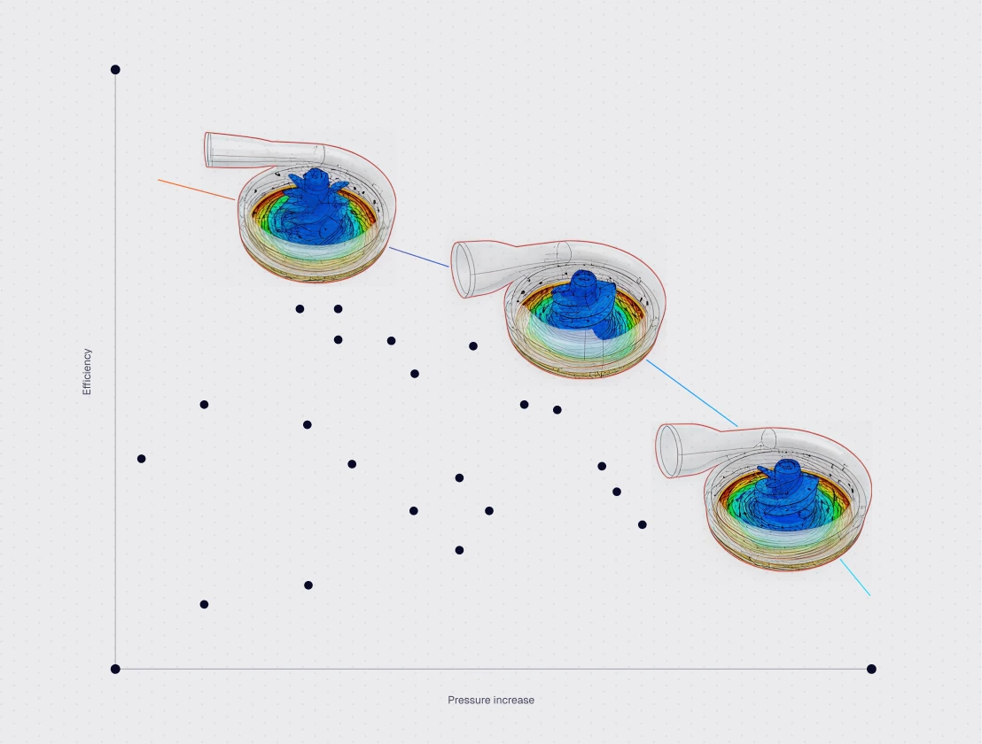
KSB ran a pump study of 377 design variants, more than 900 simulations in total. It finished in 42.4 hours and cost about $300 in compute, because the runs went out in parallel instead of one after another.
Run your first parametric experiment for free
The Community plan is free and gives you 16 cores, 10 simulations and 3,000 core hours in the browser, enough to set up a parametric experiment and see how the parallel batch behaves. No installation, no hardware, no credit card.
What design of experiments means in simulation
Design of experiments is a structured method for choosing which simulations to run so that a fixed run budget explains as much of the design space as possible. You pick the input variables you’re allowed to change, the values they can take, and the outputs you care about. The design tells you which combinations to actually solve.
Four terms carry the method:
- Factors: the inputs you vary. Blade exit angle, wall thickness, inlet mass flow, fin pitch.
- Levels: the discrete values each factor takes. Three levels of blade angle, five mass flow rates.
- Responses: the outputs you measure. Head, efficiency, pressure drop, peak temperature, maximum von Mises stress.
- Interactions: the cases where two factors together do something neither does alone. Fin pitch might help at low flow and hurt at high flow.
Interactions are the reason DoE exists. Changing one factor at a time, holding everything else fixed, is cheaper to plan and it will find a local improvement. It cannot find an interaction, because it never varies two things together. Engineers who run one-factor-at-a-time studies on coupled systems tend to discover this late, usually when a design that tested well in isolation underperforms on the bench.
For a deeper treatment of trading competing responses against each other, see multi-objective optimization.
Why sequential compute shrinks the design
Run count grows multiplicatively. A full factorial on 3 factors at 5 levels is 125 runs. Add two more factors and it’s 3,125.
Put a real solver time against that. At 4 hours per CFD run, 125 runs is 500 core hours, which on one workstation is about three weeks of continuous solving with nothing else queued. 3,125 runs is more than a year.
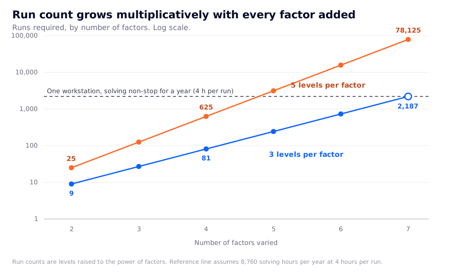
So the design gets cut. Factors get dropped on intuition, which is exactly the intuition the DoE was supposed to test. Levels get reduced to two, which makes any nonlinear response invisible. The study still produces a report, and the report is a straight-line fit through a curved design space.
Cloud parallelism reduces the wall-clock time rather than the run count. The compute bill stays roughly the same because you’re buying the same core hours either way. What changes is that they’re spent at once. KSB’s campaign hit a parallelization factor of 14, turning 25 days of cumulative solver time into 42.4 hours of waiting.
Which DoE designs parallelize well
Not every DoE design benefits equally, because some are built to run in sequence by construction.
| Design | Runs for 5 factors | Good for | Parallel behavior |
|---|---|---|---|
| Full factorial | 3^5 = 243 at 3 levels | Complete interaction mapping, few factors | Every run known upfront. Launches at once. |
| Fractional factorial | 16 to 32 | Screening many factors cheaply | Fully parallel. The standard first pass. |
| Latin hypercube | Set by you, often 10x factor count | Space-filling for surrogate model training | Fully parallel, arbitrary batch size. |
| Taguchi orthogonal array | 18 to 27 | Insensitivity to noise factors | Fully parallel. Compact and rigid. |
| Central composite (RSM) | 27 to 43 | Fitting a quadratic response surface | Fully parallel once the design is fixed. |
| Adaptive or Bayesian | 20 to 60 | Finding an optimum with fewest runs | Poor. Each batch depends on the last. |
Adaptive methods use fewer total runs, which is the right objective when compute is the scarce resource. When compute is wide and cheap and calendar time is what you’re short of, a space-filling design that runs all at once often gets you a usable answer sooner, even though it burns more core hours doing it.
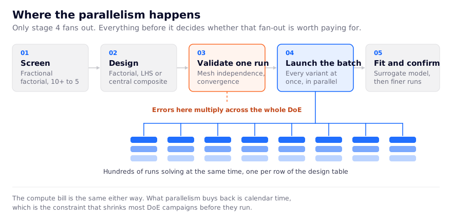
A practical sequence for most projects: fractional factorial to screen 10 or more factors down to the 4 or 5 that move the response, then a Latin hypercube or central composite design on the survivors, then a surrogate model fit to that data.
How to run a simulation DoE at scale
- Fix the response before the factors. Write down the single number that decides whether a design is better. Head at duty point. Junction temperature. Pressure drop at rated flow. A DoE with a vague objective produces a dataset nobody can act on. Secondary responses are fine to record, and they’re cheap once the run is happening anyway.
- Screen the factors. List every geometric and operating variable that could plausibly matter, then run a fractional factorial to find out which ones do. KSB parameterized 14 design variables in CAESES for the pump campaign. Screening tells you which of those deserve a fine sweep and which can be pinned.
- Parameterize the CAD properly. Most campaigns fail here. Every variant has to regenerate as valid, meshable geometry across the whole factor range, including the corners where two factors are both at their extremes. Test the extreme combinations by hand before you launch anything. A parameterization that breaks at variant 200 wastes the runs behind it in the queue.
- Pick the design and write out the run table. Factors as columns, one row per run. This table is the experiment. It’s also what you’ll join the results back onto later, so keep the variant IDs stable.
- Validate one run end to end first. Mesh independence, convergence, and a sanity check against a hand calculation or a known operating point. Run this on the baseline geometry and one extreme variant. Every modeling error left in place here gets multiplied by the size of the DoE.
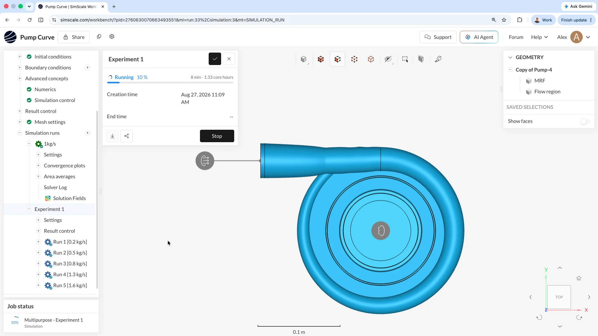
- Launch in parallel. In SimScale, a parametric experiment sweeps a table of values and launches one run per configuration, so the batch goes out together rather than queuing. This is where the cloud scale comes in, since all of those runs can execute concurrently with no need to queue them up. For the exact click path, follow how to run parametric studies in SimScale.
- Define result controls before launch, not after. Set the probes, surface integrals, and field averages you want as part of the setup. SimScale compiles those across every run in the experiment into a single plot. Skip this step and you will spend the time gathering the data afterwards instead.
- Fit a surrogate and search it. With a few hundred sampled points, fit a response surface or a machine learning model to the input-output data, then search that model instead of running more simulations. KSB built surrogate models in CAESES using its RSMtools feature. Searching a fitted surface takes seconds, and it tells you where to spend a second, smaller batch of real runs to confirm the candidate.

Andrzej Tunkiel
Mechanical Team Lead, Easee

“Due to the cloud-native nature of the solvers, the simulation speed is essentially a non-issue because I can add on more cores for faster simulation as needed. I can run 1, 2, or 20 simulations in parallel without worrying about hardware needs.”
Worked example: 377 pump variants for $300
KSB, a pump manufacturer, ran a design exploration on a heat circulator pump with CAESES handling parameterization and SimScale solving. The published figures:
- 14 design variables parameterized for CAD variation
- 377 design variants, at 3 flow rates each (0.7, 0.85 and 1.1 x Q/Q_opt), giving 900+ simulations
- 9 output parameters per variant: head, efficiency and power for the 3 flow rates
- 25 days cumulative runtime if the runs had gone sequentially
- 42.4 hours actual parallelized runtime
- Parallelization factor of 14
- 3,084 core hours, roughly $300
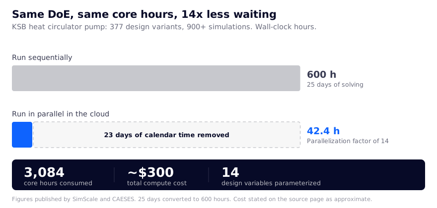
The ratio matters more than the absolute figures. For a pump program, $300 of compute is not a budget constraint, while 25 days of solving is a schedule constraint. Removing the schedule cost is what makes it reasonable to run the full design instead of a reduced one.
What parallel design space campaigns return
Rimac Automobili ran 30 thermal simulations in parallel across 10 parameter variations on a battery module. Total run time 13 hours against roughly 300 hours sequential, a 96% reduction in wall-clock time. The number of parameters you can afford to vary is set by economics rather than by hardware once the runs go out in parallel. (Rimac case study)
Allegro Energy varied fluid channel design, channel width and depth, corner radii, and the number of bifurcations and inlets across hundreds of simulations. Ryan Murphy, Mechanical Engineer: “We were able to really take advantage of the cloud scale here and look at a lot of options and combinations. In the end we increased the flow uniformity by over 40%, which has a big impact on overall efficiency as well as resulting in a better engineered and higher quality product” (Allegro Energy case study)
Crestline Coach ran 16 design iterations in concurrent batches on ambulance HVAC, varying inlet offset and angle. (Crestline Coach case study)

Bihara Singh
Automotive HVAC Product Engineer, Crestline Coach

“The ability to run simulations in concurrent batches allowed the entire virtual development process to be completed in just three to four weeks, in between other work, a fraction of the months it would have taken to build and test physical prototypes.”
In all three cases the design space got sampled at a density a sequential queue would not have allowed inside the schedule.
DoE data is training data
A well-sampled DoE produces something more durable than a winning variant: a structured dataset mapping geometric and operating inputs to simulated performance. That’s exactly the input a surrogate or machine learning model needs.
Convion, which builds solid oxide fuel cell and electrolyzer systems, ran a large design of experiments campaign in the cloud on SimScale, hundreds of simulations in parallel, and used the resulting dataset to train a Physics AI model. The model predicted performance within 5% of high-fidelity CFD and returned new candidate designs in under an hour. Armin Narimanzadeh, Manager of Thermofluids and Simulations, on the starting point: “Key performance metrics are inherently coupled and often compete with one another, creating a highly non-linear design space that we need to carefully and thoroughly explore to identify optimal solutions.”
Convion tested two approaches. First a conventional one-shot optimization loop driven by CFD simulations. Then they mapped the whole design space through DoE, trained a Physics AI surrogate model on it, and used that model to drive a second optimization study. Both workflows took the same overall time and both arrived at the same design. That makes the second one the better investment, because it leaves behind a reusable asset: with the model trained, optimizing for a new operating point in the same design space takes under an hour instead of months.
It also changes how the design should be chosen. If a campaign’s output is going to be a model, the design should be chosen for coverage of the input space rather than for the fewest runs to an optimum. That argues for space-filling designs, wider factor ranges, and keeping the runs that fail to perform, because a model learns from those too.

Armin Narimanzadeh
Manager, Thermofluids & Simulations, Convion

“We now have an AI model that can generate a new optimized design in under an hour, and I have complete confidence in the results.” Convion case study and Physics AI
Five ways a parallel DoE budget gets wasted
- Launching before validating one run. A wrong turbulence model, an unconverged mesh, or a bad boundary condition scales perfectly across 400 runs.
- Sampling infeasible corners. If two factors at their extremes produce geometry that won’t mesh, those runs fail and the design has holes exactly where the interactions live.
- Too many levels on a monotonic factor. If a response rises steadily with wall thickness, 7 levels buy almost nothing over 3. Spend the runs on the factor that curves.
- No result controls defined upfront. Post-processing hundreds of runs by hand costs more engineer time than the simulations cost in compute.
- Treating the DoE as the answer. A DoE maps the space. Confirming the chosen design usually needs a finer mesh, transient physics, or a structural check the screening runs skipped.
Frequently Asked Questions
Design of experiments is a structured way of choosing which simulations or tests to run so that a fixed run budget reveals as much as possible about how inputs drive outputs. In simulation, factors are typically geometric dimensions and operating conditions, and responses are solver outputs like pressure drop, efficiency, temperature, or stress.
A parametric study sweeps one variable across a range of values. A DoE varies several factors together according to a statistical design, so it can separate main effects from interactions. A parametric study is effectively a one-factor DoE.
For screening, roughly 2 runs per factor using a fractional factorial. For fitting a response surface, 10 or more runs per surviving factor. Five screened factors typically means 16 to 32 screening runs and 50 or more runs for a usable surrogate model.
Yes, and the number of factors rather than the run count is usually the limit. Cloud parallelism removes the wall-clock penalty, so a 243-run full factorial finishes in roughly the time of its slowest single run plus queueing. The practical constraint is that run count still grows multiplicatively, so screening first is worth the runs it costs.
Yes. The method is physics-agnostic. Factors become wall thicknesses, rib layouts, fillet radii, or load cases, and responses become peak stress, deflection, or natural frequency.
Conclusion
Screen the factors first, validate one run properly, then launch the whole design table at once. The calendar time that saves is better spent confirming the chosen design than waiting on a queue.