What is Large Eddy Simulation (LES) in CFD?

Turbulent flow often requires substantial computational power to simulate accurately. CFD simulations simplify the problem to reduce computing time while maintaining or improving accuracy. Large Eddy Simulation (LES) is one of those CFD techniques that balances detailed simulations with manageable computing demands.

In this article, we’ll explore LES in detail – what it is, how it differs from other CFD models, and why it’s often the best choice for certain simulation needs. We’ll also discuss its practical applications and how it is implemented in SimScale.

Key Takeaways

• LES prioritizes larger eddies influenced by flow geometry, using a subgrid-scale model for smaller, more universal scales.
• LES is ideal for capturing transient turbulent structures, unlike time-averaged RANS models.
• LES has a wide range of applications, from aerospace aerodynamics to urban planning and marine engineering.
• SimScale’s user-friendly tools make LES more accessible, especially for small to medium-sized enterprises.

What Is Large Eddy Simulation?

Large Eddy Simulation (LES) is a mathematical model for simulating turbulent flow in computational fluid dynamics. It’s particularly valuable in sectors like aerospace and automotive, where understanding how fluids interact with various structures is critical. The roots of LES trace back to 1963, when Joseph Smagorinsky proposed it to simulate atmospheric air currents. Its first significant exploration was by Deardorff in 1970.

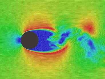
LES focuses on larger eddies (whirls of fluid) in a flow, influenced by the geometry of the flow, while the smaller, more universal scales are modeled using a subgrid-scale (SGS) model. This methodology stems from Kolmogorov’s 1941 theory of self-similarity, which suggests that larger eddies are shaped by flow geometry, whereas smaller scales are more universal.

Navier-Stokes Equation: The Basis of LES

At its core, LES deals with fluid behavior using the Navier-Stokes equations, which are fundamental in fluid dynamics. These equations cover three main areas:

• Conservation of Mass: This principle states that the total mass of the fluid remains constant, no matter how it moves or changes shape.
• Conservation of Momentum: Based on Newton’s second law, this aspect ensures that the momentum within a fluid system remains constant over time.
• Conservation of Energy: Here, the total energy of an isolated system is conserved, following the first law of Thermodynamics.

Now, let’s talk about the filtering kernel in LES. This filtering process is crucial for LES because it simplifies these complex Navier-Stokes equations.

The kernel works by focusing on the larger eddies in the fluid, which are the main drivers of flow patterns in turbulence, and averages out the effects of the smaller eddies. This is done through a mathematical operation known as convolution, which blends the fluid’s characteristics over a particular scale.

The filtering operation in Large Eddy Simulation (LES) is generally expressed in the following integral form:

$$ \bar{\phi} (x,t) = \int_{-\infty}^{+\infty} \int_{-\infty}^{+\infty} \phi (r,\tau)G(x-r, t-\tau)drd\tau $$

where:

• \(\bar{\phi} (x,t)\) is the filtered field variable, which could represent quantities like velocity or pressure at a point \(x\) and time \(t\).
• \(\phi (r,\tau)\) is the unfiltered field variable at position \(r\) and time \(t\).
• \(G(x-r, t-\tau)\) is the filtering kernel applied to the field variable.
• The double integral indicates that the filtering is applied over all space and time, with \(dr\) and \(d\tau\) being the differential elements for integration.

After filtering, the field variable is split into two parts:

• Filtered Component (\(\bar{\phi}\)): This is the larger-scale part of the flow, which the LES filter keeps. It represents the averaged effect of the flow across larger eddies and structures.
• Subgrid Scale Component (\(\phi’\)): This is the smaller-scale part that the LES filter doesn’t directly compute. It includes all the tiny eddies and fluctuations that are too small to be captured by the filter.

Together, the total field variable is described as the sum of both the filtered and subgrid components:

$$ \phi = \bar{\phi} + \phi’ $$

LES for Compressible & Incompressible Flows

The LES-filtered Navier-Stokes equation for an incompressible fluid flow, which assumes constant density and no divergence, is shown below. In Einstein’s notation, it is:

$$ \frac{\partial \bar{u_i}}{\partial t} + \frac{\partial}{\partial x_j}(\bar{u_i}\bar{u_j}) = -\frac{1}{\rho} \frac{\partial \bar{p}}{\partial x_i} + \nu \left(\frac{\partial^2 \bar{u_i}}{\partial x_j^2} + \frac{\partial^2 \bar{u_j}}{\partial x_i^2}\right) $$

The LES approach for compressible flow involves additional considerations for density changes.

$$ \frac{\partial \bar{\rho}u_i}{\partial t} + \frac{\partial \bar{\rho}u_i u_j}{\partial x_j} + \frac{\partial p}{\partial x_i} – \frac{\partial \bar{\sigma_{ij}}}{\partial x_j} = – \frac{\partial \bar{\rho} \tau_{ij}}{\partial x_j} + \frac{\partial}{\partial x_j}(\bar{\sigma_{ij}} – \bar{\bar{\sigma_{ij}}}) $$

The filtered motion equation for compressible flow within LES accounts for variations in fluid density and includes modifications to the stress terms to reflect the fluid’s response to being compressed. This variant of the motion equation is often referred to as the Favre-averaged Navier-Stokes equation.

When to Use Large Eddy Simulations in CFD

Large Eddy Simulation (LES) is your go-to computational fluid dynamics (CFD) model when the flow’s transient and turbulent structures are critical to capture. Unlike steady models, such as the Reynolds-Averaged Navier-Stokes (RANS) turbulence model, which offers time-averaged results, LES can detail the fluctuating components of turbulence that evolve over time.

In many complex flow scenarios, RANS models fall short as they cannot accurately represent the entire flow field, especially when the turbulent fluctuations are not just minor disturbances but significant enough to influence the mean flow.

LES vs. RANS vs. DNS

Here are the key differences between LES, RANS, and DNS mathematical models:

Feature	DNS	LES	RANS
Applications	Simple flow, low Re number	Simple flow, low Re number	Wide range
Computational Power	Very high demand	Less demand than DNS, higher than RANS	Least demand
Accuracy	Most accurate	More accurate than RANS, less than DNS	Least accurate
Complexity	Can’t handle complex systems due to computational load	Handles more complexity than RANS	Can handle complex systems
Turbulence	Resolves all scales of turbulence	Resolves large scales, models small scales	Models all scales of turbulence
Suitability	Academic and theoretical studies	Flows with significant large-scale turbulence	Industrial and practical applications where efficiency is key
Cost	Prohibitively high for most practical applications	High but more feasible than DNS	Economical and practical
Typical Use Case	Fundamental research, low Reynolds number flows	Transitional and complex turbulence not suited for RANS	Flows where turbulence is well-behaved and predictable

Applications of Large Eddy Simulations

Here are some key areas where LES is making a significant impact:

• Aerodynamics and Aerospace: LES is used to study a wide range of aerodynamic and aerospace problems, including turbulence in aircraft wakes, flow around buildings and structures, and combustion in military and aircraft aircraft engines.
• Automotive Engineering: Car manufacturers rely on LES to optimize aerodynamics for better fuel efficiency and stability.
• Geophysics and Environmental Engineering: LES can solve geophysical and environmental problems, by studying atmospheric turbulence, ocean circulation, and transport of pollutants in the atmosphere and ocean.
• Industrial Applications: Simulating flow in heat exchangers, combustion in furnaces, and flow around turbines, motors, and pumps.
• Marine Engineering: LES is critical for studying the interplay between water currents and ship hulls.

Challenges of Using LES

Current Challenges of LES

• Computational Resources: Although less demanding than DNS, LES requires significant computational power, especially for flows with high Reynolds numbers or complex geometries.
• Boundary Conditions: Implementing accurate boundary conditions for LES can be complex, as it must capture the inflow turbulence characteristics correctly.
• Computational Cost: Despite advances in computational hardware, the cost of running LES can still be prohibitive, especially for small to medium-sized enterprises.
• User-Friendly Tools: Developing more user-friendly LES tools that require less expertise to set up and interpret is necessary to make LES accessible to a broader engineering community. This is where SimScale makes advanced simulations more accessible to engineers and designers who may not have specialized knowledge in turbulence modeling.

Future Challenges of LES

• Integration with Machine Learning: As machine learning algorithms become more prevalent, integrating these methods with LES to improve subgrid-scale models is both a challenge and an opportunity.
• Multi-Physics Coupling: Many real-world applications involve coupling between turbulence and other physical phenomena, such as heat transfer or chemical reactions. Developing robust LES strategies for multi-physics problems may be challenging.
• Data Handling and Storage: The vast amounts of data generated by LES simulations present challenges in terms of storage, processing, and data mining for insights. This is where cloud-native simulation like SimScale would be perfectly fitting, as users can leverage the relatively infinite storage capacity in the cloud.

Large Eddy Simulations on SimScale

SimScale takes the complexity out of running Large Eddy Simulations (LES). Here, you can explore the behavior of simple laminar flows and more complex turbulent flows.

With SimScale’s entire cloud-native platform operating directly through your web browser, you’re free from the constraints of computing power, accessibility issues, and the steep costs typically associated with advanced simulations. By relying on cloud computing capabilities, you are able to run as many simulations as you need simultaneously without hardware constraints. You can also access your simulation projects anytime and anywhere by simply tapping into your web browser.

Applying LES in SimScale

LES is one of many turbulence models that can be simulated in SimScale, such as the K-epsilon, K-omega, and K-omega SST models. By applying LES, the smallest scales of turbulence would be spatially filtered out to be modeled, and the largest, most energy-containing scales would be resolved by the mesh. Such a method allows for relatively coarse mesh resolution (compared to DNS), which makes it more widely applicable to different types of fluid flow problems.

SimScale offers three LES turbulence models, namely:

• LES Smagorinsky: Subgrid-scale turbulence model in LES that introduces a constant viscosity term to account for unresolved turbulent structures
• LES Spalart-Allmaras: One-equation LES turbulence model simplifying computations by solving for a single variable, the turbulent viscosity, to model various turbulence effects
• LES Smagorinsky (direct): (available only for the Incompressible LBM solver) While the Smagorinsky model strictly follows the original formulation and LES idea, the Smagorinsky (direct) is a bit cheaper, but a bit modified. For Smagorinsky Direct, only the LBM mesh has to be computed during a time step, while for Smagorinksy, the LBM and the Finite-Difference meshes have to be computed during a time step making it comparatively costlier.

Examples of LES in SimScale

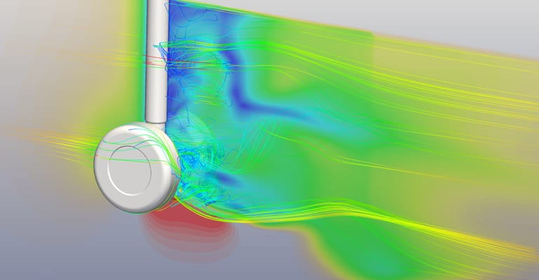
Consider the challenge of reducing the roar from an aircraft’s landing gear. This is where LES shines. On SimScale, you can map out how air whirls around the wheels and struts, ensuring the safety of the plane and passengers.

Here, the LES Smagorinski model for sub-grid scales was used after a mesh of 1.8 million nodes was applied (using SimScale’s SnappyHexMesh). The free stream flow velocity (Air) is set to be 35 m/s at standard conditions. A ramping of the velocity boundary condition was applied to gradually increase the velocity from a low value to a free-stream value for faster convergence.

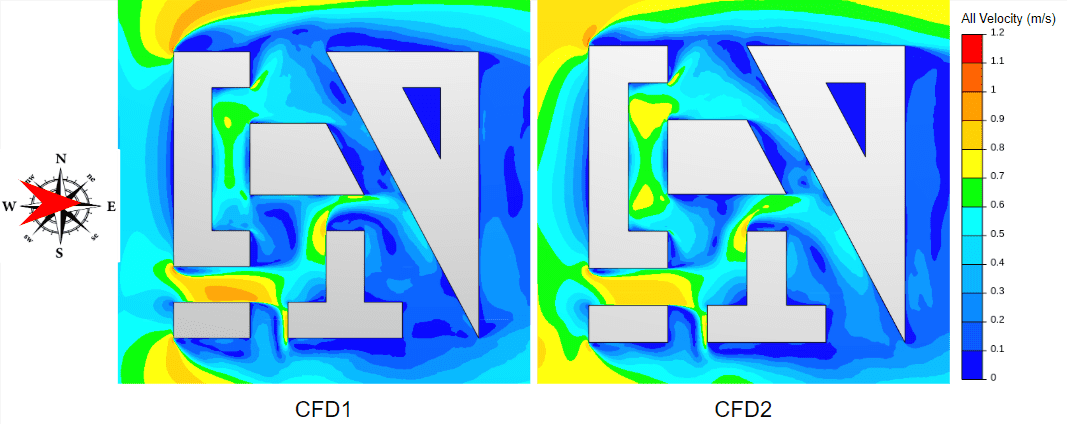
Another example explores the accuracy of SimScale’s Lattice Boltzmann Method (LBM) compared to wind tunnel tests conducted by two German institutes. The image below demonstrates this validation case, comparing the LES results from two different wind tunnel tests.

For this project, a turbulence model that combines both LES and RANS was used, called k-Omega SST (or Delayed Detached Eddy Simulation (DDES)). This method enables the simulation to switch between both LES and RANS. Based on this, the findings showed a good agreement between the simulation results and wind tunnel test results. If you are interested in the details of this comparison, read the validation case here.

Ready to see LES in action? Start Simulating on SimScale by clicking the button below and push your designs forward with confidence.

Last updated: December 7th, 2023

What's Next

What is Valve Flow Coefficient?