Documentation
This document focuses on some important aspects of the Incompressible LBM (lattice Boltzmann method) analysis type in SimScale in detail.
The Pacefish®\(^1\) LBM solver can deal with many CAD types and is generally more robust than many solvers in terms of cleanliness of the geometry, where open geometry, poor faces, and small faces don’t matter. That said, on the odd occasion you have issues or errors, if you inspect the geometry and don’t find anything fundamentally wrong, a *.stl can normally be loaded.
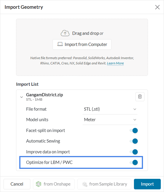
Optimize for PWC/LBM
This option allows you to import a *.stl file that is optimized for the Incompressible LBM and Wind Comfort analysis types. It leaves out complex import steps like sewing and cleanup that are not required by the LBM solver and therefore also allows importing large and complex models fast.
The Y+ requirements for LBM tend to be more robust than those of the equivalent finite volume methods, for example, the K-omega SST (uRANS) model in the FVM implementation has an approximate requirement of 30 < Y+ < 300. In the SimScale’s LBM implementation the lower bound is not considered a requirement and instead a more robust upper bound of less than 500 and certainly not higher than 1000 is recommended. The solver will additionally warn for Y+ values higher than 2000 in the near-wall voxel.
If the Y+ is much higher than expected where results are likely to be impacted the user will be warned in the interface as follows:
Warning
High velocities encountered that might not be handled by the current mesh resolution. Please check your results and consider refining the mesh further.
OR
Mesh resolution might not be sufficient for correct turbulence modeling. Please check your results and consider refining the mesh.
And in the solver log with an error:
Warning
ERROR @ DomainHealthStatusExporter.cpp:60: simulationTime=748, domainHealthStatus=(maxVelMag=0.323367, minRho=0.697381, maxRho=1.48795, maxNuT=0.000625238, maxWallCellSizeYp=102696)
The warning message above shows a maximum Y+ of 100k which is very high and needs to be reduced. The main methods of doing this involve the application of Reynolds scaling (see the section below) or refining the surface mesh. If the surface is already refined to a reasonable level, scaling is the only option without excessively increasing the cost of your simulation.
Regarding Y+ targets, Pacefish®\(^1\) is much more flexible than FVM codes with wall functions. It has no limitation regarding the low-bound value. The results should not suffer from wall resolution as long as the size of the wall-next voxels is not exceeding 500 to 1000.
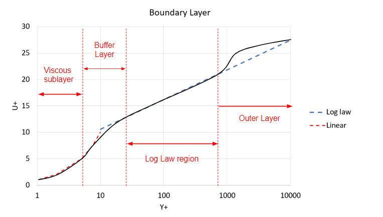
From Figure 2 we can see the different regions of the boundary layer and why when modeling the layer it’s encouraged to avoid the Log Law Region. However, K-omega SST models the layer up until the first cell and then solves from there on, and this model has been proven to be very accurate in many industries including the aerospace industry.
Although the K-omega SST model is highly accurate, more accurate models exist, namely LES (Large Eddy Simulation) and DES (Detached Eddy Simulation).
LES is more accurate as it models only eddies smaller than the grid filter and solves the flow regime larger than the grid filter size. Amongst its downfalls is its inability in its standard form to model walls, therefore requiring a very fine mesh, or simply dealing with flows where wall interactions are least predominant. Pure LES models such as the ‘LES Smagorinsky’ model require similar Y+ requirements to the equivalent FVM model, where Y+ is around or below 1. This is one of the main reasons LES will be a more expensive simulation.
However, if a wall model were to be added, we could obtain the accuracy improvements without the requirement of such a fine mesh, and this is where the advantage of DES or Detached Eddy Simulation comes in.
Smagorinsky (direct) turbulence model
Besides the traditional Smagorinsky model, SimScale also offers Smagorinsky (direct) turbulence model.
“Smagorinsky” model strictly follows the original formulation and LES idea. “Smagorinsky (direct)” is a bit cheaper, but a bit modified. For “Smagorinsky Direct” only the LBM mesh has to be computed during a time step, while for the “Smagorinksy” the LBM and the Finite-Difference meshes have to be computed during a time step making it comparatively costlier.
DES turbulence models are a hybrid LES-uRANS model that uses RANS formulation in the boundary layer and LES formulation in the far-field achieving an optimum between both worlds. In the LBM solver, two detached eddy models are available, the K-omega SST DDES (Delayed Detached Eddy Simulation) and the K-omega SST IDDES (Improved Delayed Detached Eddy Simulation).
The DES models ‘K-omega SST DDES’ and ‘K-omega SST IDDES’ have similar wall requirements to the uRANS ‘K-omega SST’ since the wall model is based upon the same model however, at some point the near-wall region transitions from K-omega SST to LES.
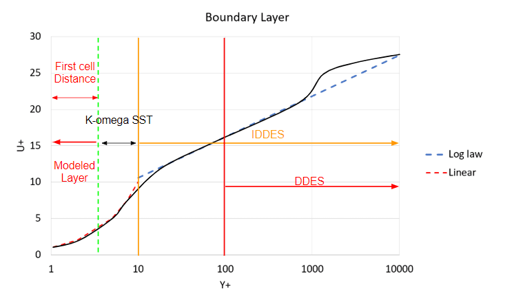
The difference between DDES and IDDES is that IDDES blends from uRANS to LES in the buffer region which can be approximated to be somewhere between 5 < Y+ < 30, whereas the DDES model blends from uRANS to LES in the log-law region 30 < Y+. Therefore, depending upon the Y+ values of your mesh choose the appropriate DES turbulence model. For example, if your Y+ is around 100, then the DDES model would be better, however, if the Y+ is below 5, the IDDES would be more suited than DDES.
Since the K-omega SST model probably swallows some of the transient effects and you are tempted to use the plain Smagorinsky model, make sure that wall resolution has to be around or below Y+ of 1.’ – (Eugen, 2018)\(^1\). However, when you are simply rerunning the simulation for improved results without refining the mesh please consider using the DES turbulence models available in SimScale instead of the plain K-omega SST and Smagorinsky models.
It is common to scale down a model physically for wind tunnel testing or to slow down a flow or change other flow parameters. Examples of such a requirement include testing a scaled building or a plane in subsonic flows. In SimScale, the Reynolds scaling factor (RSF) can apply this scaling automatically to a full-scale geometry.
Not only is this scaling important in wind tunnels for obvious sizing reasons, but it is also required in the LBM method, where a high Reynolds number will create a thin boundary layer which will also need a finer mesh to compensate. Since the LBM requires a lattice where the aspect ratio is 1, a perfect cube, refining to the required Y+ values may become expensive. On top of that, if you were to refine to the required level at the surface without scaling, then because the Courant number is being maintained at a value lower than 1, the number of time steps required for the same time scale would increase further increasing the simulation expense.
The depicted validation case, AIJ Case E, for pedestrian wind comfort is compared to a wind tunnel where the scale of the city is 1:250, and a scaling factor of 0.004 could be used. Alternatively, we can use auto meshing where the Reynolds scaling factor is applied automatically. If dealing with a high Reynolds number it is recommended that some literature review is used to understand an acceptable scaling factor for the application, or if in research, choose the matching scale factor to the wind tunnel you are comparing to.
The Reynolds scaling factor can be accessed under Mesh settings, for both Incompressible LBM and Pedestrian Wind Comfort analyses:
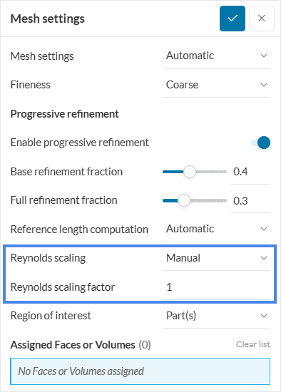
The Reynolds number is defined as \(Re = U L/ \nu\) where \(L\) is the reference length, \(U\) is the velocity, and \(\nu\) is the kinematic viscosity of the fluid. When a scaling factor is applied, instead of sizing the geometry down, the viscosity is increased to ensure that the Reynolds number is reduced to the correct scaling.
In most urban scale flows, an Automatic Reynolds scaling is recommended to ensure accurate results. Like wind tunnel models, we use Reynolds scaling assuming that bluff bodies (block-like buildings) and high Reynolds numbers are present. This enables the concept of similarity of large Reynolds numbers. When both these conditions are met, automatic scaling is valid. Automatic Reynolds scaling helps you get accurate results, cheaper without extensive expertise.
Advanced users operating outside the typical assumptions of urban scales are welcome to use manual scaling, however, they should consider the impacts on wall modeling and rely on their expertise. A scale of 1 represents full scale, 1/250 or 1/400 would represent a typical wind tunnel scale. Automatic values in SimScale are typically in the order of 1/10.
We applied a simple rule of thumb where the mesh of the worst resolved solid is still a maximum of two refinement levels below the best resolved solid. Because memory consumption scales with second order and computation effort scales with third order you already will have a huge saving compared to resolving all solids at the highest refinement level (93% less memory and 99% less computation time), but at the same time have stable (not-changing) resolution at the wall getting rid of numeric effects at the transitions.
Please consider grid transition at solids an expensive operation in terms of results quality even if no computation errors occur and you do not directly see the effects. This means you can use it, but do it carefully. It is best to maintain the same refinement level for solids as far as possible.
If the above rule of thumb is followed using a VoxelizedVolume with a unidirectional extrusion size of 4 voxels and directional downstream extrusion of 16 voxels, then you will get very good geometry-adapted meshes being a lot better suited for the simulation in almost any case than those refinement regions build of manual boxes. Generally, consider refinement boxes a tool from the Navier-Stokes world. They still work for Pacefish, but VoxelizedVolumes work much better.
Ordinary Finite Volume Method-based solvers usually run in the steady-state, and usually on grids sub 20 million, so saving the entire results for the final step is no issue. However, on the LBM solver, it’s normal to have grids bigger than 100 million cells, and since it’s transient, results are computed at every time step. The size of a complete result is usually too large to realistically fully output and store.
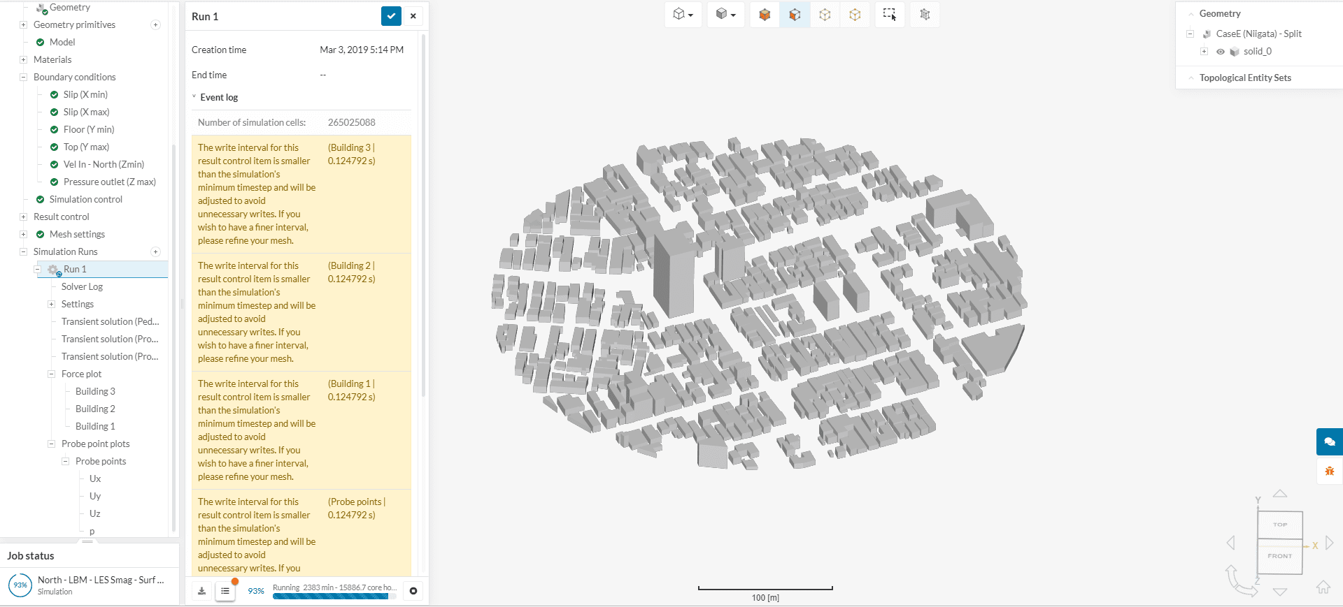
If the simulation runs out of results storage an error will start appearing in the logs:
Error
FATAL @ EnSightExport.cpp:3679: EnSight data export to “export/trans_Pedestrian__PACEFISHSPACE__Level__PACEFISHSPACE__SlicePACEFISH” FAILED because of file I/O issue. Please check the access rights and the available disk space at the destination.
If this starts appearing it is advised to immediately stop the simulation and re-adjust the result controls to reduce the size of the written data, as any further produced data is unlikely to be written, and therefore further solve time will not gain you additional results and only waste GPU hours.
Predicting the amount of data written is not an exact science as the results depend upon the mesh size, the export domain size, the frequency of transient result write, and the time a simulation is run for. So, although it might be hard to judge, simply being conservative, realistic, and putting thought into what you need at the end of a simulation will likely produce simulation results without error.
Example 1
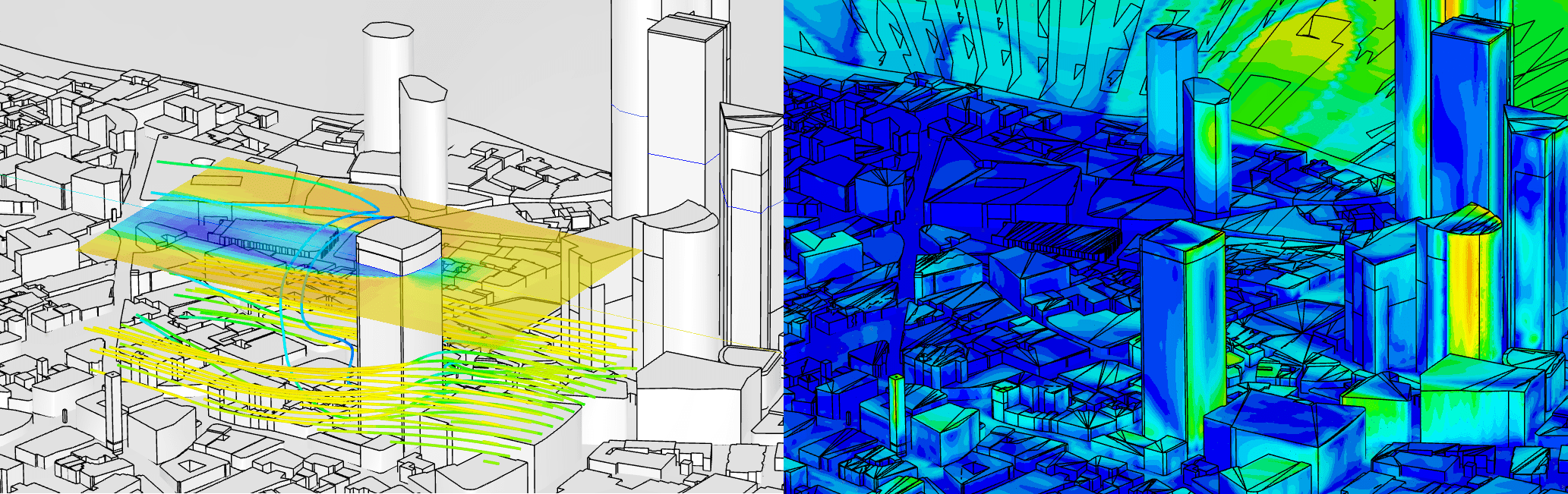
If you are interested in peak velocities at various points at pedestrian height in a city, you could simply export transient data of the encompassing area, however, to get good transient results many writes will be needed, and realistically, at every time step. This won’t be practical for a well-refined domain exceeding 100 million cells with appropriate wall refinements. An alternative would be to save a region much smaller, such as a slice with a small region height drastically reducing the size of the results.
We could be even more conservative, we could know the points of interest and upload these points as a CSV file and export them every time step.
Example 2
In wind loading, where you simply want to understand pressures on the surfaces of the building, you could export fluid and surface data around a city, or reduce it to just the building of interest. Furthermore, we could remove the volume data and only export surface data reducing the size of the results to two dimensions.
In the above two examples, it is up to the user to determine the level of results they require, however, every time you drop a level a significant amount of additional storage space becomes available, leading to highly productive simulation runs.
For this reason, the LBM allows three main methods of result exportation: Transient output, Statistical averaging, and Snapshot. Let’s go through these three options:
With this result control item, transient results can be saved for a given part of the simulation run, for a given output frequency, for a desired region within the fluid domain. The settings panel looks as follows:
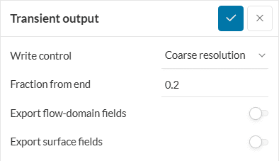
The following parameters need to be specified:
Note
Transient results are recommended to be saved for small domains especially if an animation is desired. If your simulation runs out of memory, your simulation will fail, wasting potentially a lot of solve time. So be conservative with the transient output and think about the exact results you need.
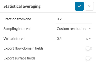
With this result control item, the average of the exported transient output will be calculated for a given fraction from end. For example, for a fraction from end of 0.2, the average of each field value within 20% from the end of the simulation will be computed.
We can’t take every time step for the calculation of the average, as this would be computationally too expensive. Hence, to make the computation effort feasible, we use the Sampling interval that stores results only every 2nd, 4th, or 8th time step (besides custom resolution) for the averaging.
The rest of the filters in the settings panel are the same as that for the transient output discussed above.
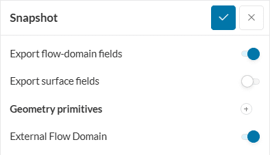
With this result control item, the final state of the transient results can be output. That is no intermediate results can be observed except that at the final time step.
As obvious there are no write filters:
This result control item allows calculating forces and moments in the course of the simulation by integrating the pressure and skin friction over a boundary. It is possible to select a set of boundaries to calculate the overall force and moment on them.
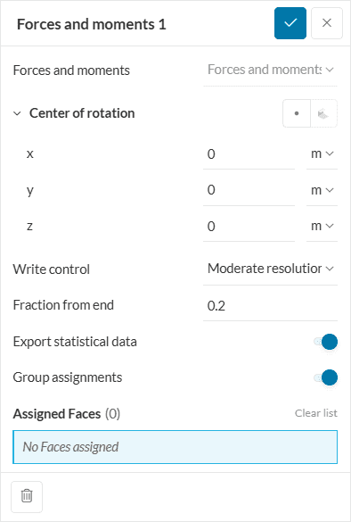
The following parameters need to be specified:
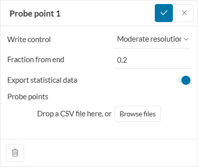
Probe points are useful as velocity measuring devices (virtual hot wires or pitot tubes) or can be added to monitor pressure at a point (virtual pressure tap points) where data for each probe is returned as components of velocity and pressure. Additionally, statistical data on those points can also be exported in the form of a sheet.
The format for specifying the probe plot is:
Label, X ordinate, Y ordinate, Z ordinate
Where an example is:
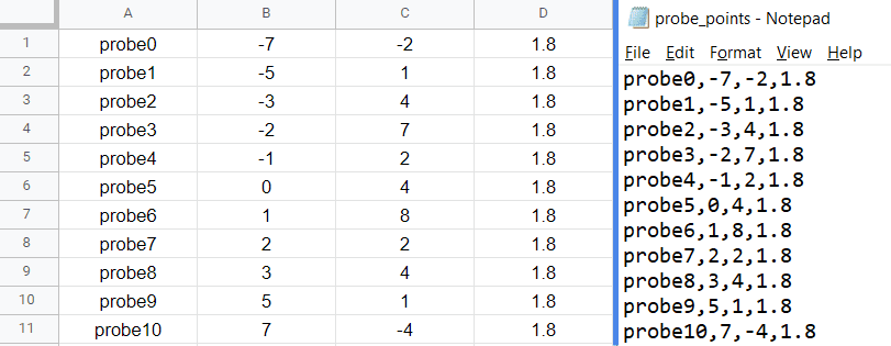
This can easily be done in a notepad (.txt), Excel, or your choice of spreadsheet software which can export in .csv format.
Maximum number of Probe points
If any of the above limits are exceeded the user will receive an error.
Time steps bigger than the export frequency
It is important to note that if the time steps are bigger than the export frequency, then the data is returned at the rate of the time step size, and the user is warned in the user interface. This is important if doing a spectral analysis with a different frequency than the export frequency in the interface. This is true for all the result control items.
References
Last updated: February 12th, 2025
We appreciate and value your feedback.
Sign up for SimScale
and start simulating now


