Validation Case: RUB Wind Tunnel Tests Validated Against Lattice Boltzmann Method-SimScale
This document provides a comparison of computational fluid dynamics (CFD) simulation results done with the lattice Boltzmann method (LBM) in SimScale with RUB wind tunnel tests conducted by two German research institutes.
Overview
Wind tunnel testing has been in use as an experimental tool to observe the effects of wind on buildings\(^1\). The use of wind tunnels is not only beneficial for the architectural industry, but also in the aviation, construction, and automotive fields. However, the rise in computational power and the development in computational analysis makes CFD a fast and cost-efficient addition to wind tunnel testing, especially in the early design stages.
Wind analysis results obtained from CFD simulation can be seen as trusted sources of qualitative and quantitative data, as they are used in making important design decisions. One method that can be employed is the lattice Boltzmann method. This method has gained popularity in the last two decades as an alternative to conventional CFD methods such as the finite volume method (FVM) and the finite difference method (FDM).
The advantages of running a simulation with the LBM method compared to conventional CFD methods are that it can handle extremely complex geometries better and its efficient parallelization in combination with the use of graphical processing units (GPUs) makes it suitable for large transient simulations. This makes LBM an attractive option, especially when combined with cloud computing, as it is becoming more accessible and powerful. The LBM solver implemented in SimScale is Pacefish\(^®\) developed by Numerics Systems GmbH.
In order to have full confidence in the simulation results, comprehensive validations and verifications of CFD results are necessary. With this in mind, at SimScale we validate all released major features by comparing the simulation results to analytical or experimental data. Therefore, in this article, we have provided a comparison of two wind tunnel results with a simulation done in SimScale using LBM.
Wind Tunnel Tests
The wind tunnel tests are based on a study done by C.Kalender with the title “Vergleich Unabhängiger Experimenteller Ausbreitungs-untersuchungen In Einem Fiktiven Stadtmodell“\(^2\).
The wind tunnel results used for validation were taken from two different institutions:
- IFI: ABL Wind Tunnel, Institut für Industrie-aerodynamik (IFI), Aachen. The experiment results from this institution will be later referred to as WT1.
- WIST: ABL Wind Tunnel, Arbeitsgruppe Windingenieurwesen und Strömungsmechanik (WIST), Ruhr-Universität Bochum. The experiment results from this institution will be later referred to as WT2.
Geometry
We used the following models taken from the wind tunnel experiments:
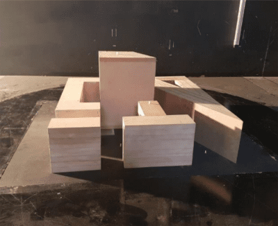
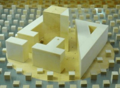
Both models have a scale of 1:200. In order to be able to validate the lattice Boltzmann solver, we recreated the scaled model as a computer CAD model and the specifications of the virtual wind tunnel size are tabulated below:
| Specifications | Size |
| Flow-parallel | 4.8 \(m\) |
| Spanwise | 3.6 \(m\) |
| Height | 1.8 \(m\) |
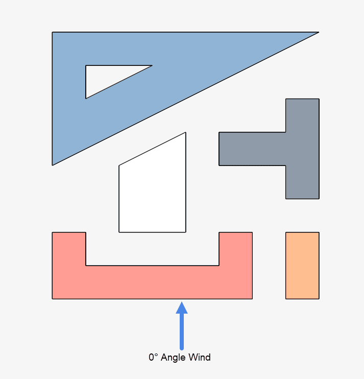
The figure below shows the CAD model used for the simulation:

Pre-Processing
The turbulence model used is k-Omega SST (DDES) so the simulation can switch between the Large Eddy Simulation (LES) and the RANS (Reynolds Averaged Navier Stokes) model. The simulation is a transient analysis for 3.6 fluid passes and the last 30% of the data are averaged for comparison with the results from the wind tunnel tests.
You can read more about fluid passes here.
Wind Direction and Measurement Points
Firstly, the wind direction used in this simulation is a 0° angle wind which can be seen below:
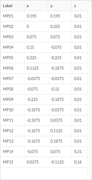
Additionally, we inserted probe points as done in the wind tunnel experiments as measurement points, and below is a table showing the coordinates of the probe points along with their names.
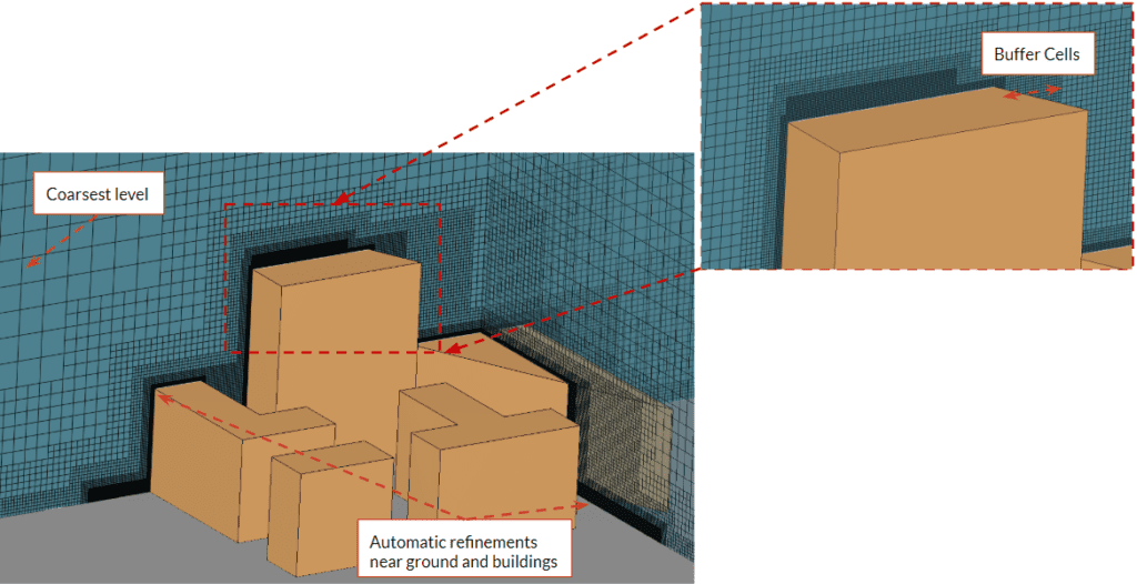
Mesh
Next, we generated the mesh using Moderate fineness level and refined with Moderate refinements at the pedestrian level (0-0.02 \(m\)) and in areas in the proximity of measurement points MP14 and MP15. The number of cells and the minimum cell size can be seen in the table below:
| Specifications | Quantity |
| Number of 3D cells | 34 Million cells |
| Minimum cell size | 0.00115 \(m\) |
Additionally, the mesh generated can be seen below:
Boundary Conditions
For this study, the reference wind speed of 10 \(m/s\) is considered at the reference height of 0.15 \(m\) for the wind tunnel model. Furthermore, the velocities were normalized by this reference velocity for all simulation results.
We ran two simulations that are based on each test and used an atmospheric logarithmic boundary layer (ABL) profile based on each test. Firstly, the specifications of each test are in the table below:
| Boundary Condition | IFI (CFD1) | WIST (CFD2) |
| Measuring system | FID/Pointwise | ECD/backsampling |
| Velocity measurement method | Spherical head probe | Heated single filament wire |
| Scale | 1:200 | 1:200 |
| Roughness length (\(z_{0[Model]}\)) | 0.0028 \(m\) | 0.0017 \(m\) |
| Offset height (\(d_{0[Model]}\)) | 0.01 \(m\) | 0.005 \(m\) |
| Exponential profile (\(\alpha\)) | 0.22 | 0.20 |
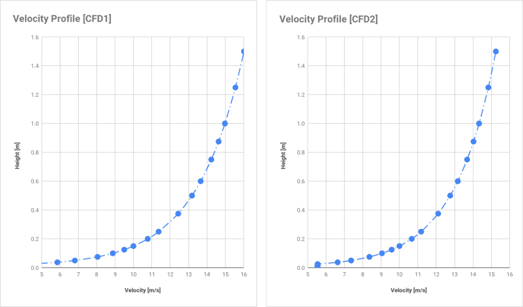
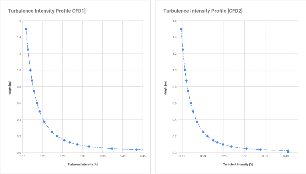
Secondly, the ABL profile for the mean velocity and turbulence intensity was calculated with the formula below:
$$U = 10 \frac{ln(\frac{d-d_0}{z_0})}{ln(\frac{Z_{ref}-d_0}{d_0})}\tag{1}$$
$$I=\frac{1}{ln(\frac{d-d_0}{z_0})}\tag{2}$$
The graphical representation of velocity profile from each experiment can be seen below:
Finally, the graphical representation of the turbulence intensity profile applied in the simulations can be seen below:
Results and Analysis
As stated before, the velocities are normalized for all results by the reference velocity. The velocity profile from each simulation and experiment is compared to observe the deviation of each result and serves as a comparison between the wind tunnel tests and simulations done with LBM.
Results Comparison
The flow visualization and velocity plot can be observed below:
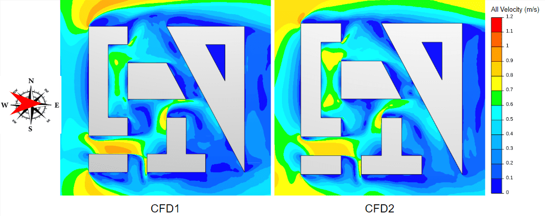
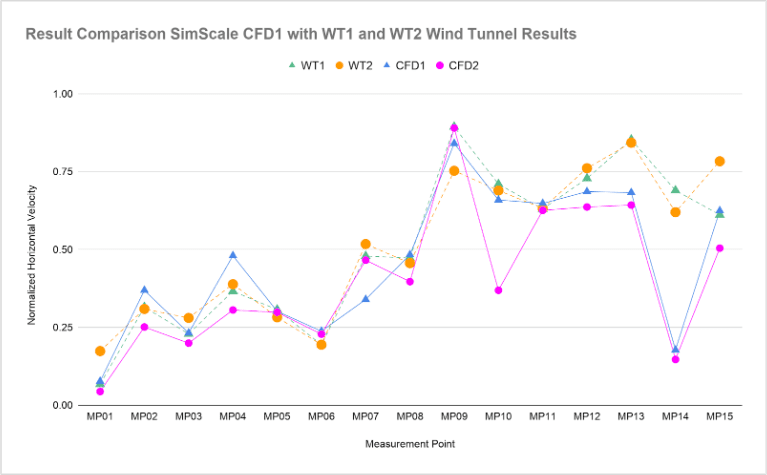
From a 0 degree angle, there is a good agreement between the simulation results and wind tunnel test results. 13 measurement points are within +/- 20 relative deviation to the wind tunnel results. The deviation from each simulation result compared to its corresponding wind tunnel experiment can be observed below:
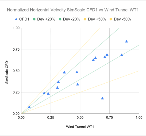
When compared with WT1, 14 measurement points are within +/- 50 relative deviation to the wind tunnel results.
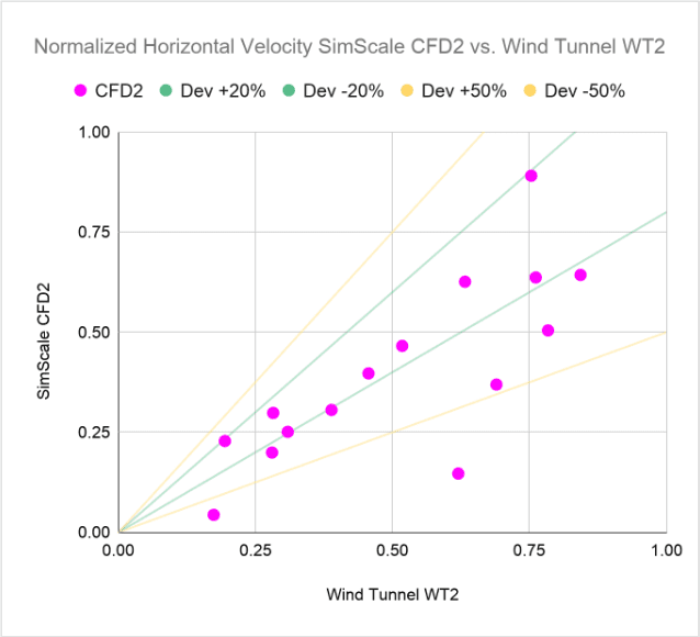
And when compared to WT2, 13 measurement points are within the +/- 50 relative deviation to the wind tunnel results.
Results Analysis
A correlation analysis between the CFD simulation and the wind tunnel tests can be described in two numbers, the hit-rate criteria and the Pearson coefficient.
| Hit-rate* | Pearson | Hit-rate** | Pearson*** | |
| 0° CFD1 – WT1 | 80% | 0.82 | 86% | 0.96 |
| 0° CFD2 – WT2 | 67% | 0.77 | 71% | 0.86 |
* Hit-rate defined according to VDI using a relative tolerance of D= 0.25 and an absolute tolerance of W= 0.06.
**/*** Hit-rate and Pearson coefficient calculated with MP14 excluded.
From the 0° angle, there is a good agreement between the CFD and wind tunnel test results because the hit-rate is higher than the criteria of 66% and a Pearson coefficient above 75%.
However, we can also see that the normalized velocity at MP14 does not agree with the wind tunnel results. This is due to the specific location of MP14 which is inside a separation region on top of the roof. The simulation results show a rather low mean velocity where the wind tunnel experiments indicate a velocity at approximately half of the freestream velocity. Possible reasons for the differences are:
- The simulation uses a steady inlet ABL profile, ignoring the transient fluctuations in turbulence and velocity at the inlet.
- The reference speed of 10 \(m/s\) might be larger than the velocity used in the wind tunnel experiments, which leads to an increased separation region.
Conclusion
In conclusion, the comparison provided above between the wind tunnel tests and simulations done with SimScale’s Pacefish® LBM solver integration produced comparable results.
References
- B. Kayışoğlu, et al.’Estimation of Wind Loads on Tall Buildings through Wind Tunnel Testing’.Oct. 2012.
- C. Kalender.’Vergleich Unabhängiger Experimenteller Ausbreitungs-untersuchungen In Einem Fiktiven Stadtmodell’.October.2019.
- Y. Lin, et al. ‘Research on Physical Wind Tunnel and Dynamic Model Based Building Morphology Generation Method’. May 2019.
- D. Phillips, et al, ‘Will CFD ever Replace Wind Tunnels for Building Wind Simulations?’.International Journal of High-Rise Buildings Volume 8 Number 2. June 2019.
- J. Zhang,.Lattice Boltzmann Method for Microfluidics: Models and Applications’.Microfluid Nanofluid 10:1-28,2011.
- Arumuga Perumal, D., Dass, Anoop K. ‘A Review on the Development of Lattice Boltzmann Computation of Macro Fluid Flows and Heat Transfer’. Alexandria Engineering Journal 54:955-971,2015.
- VDI.’VDI Richtlinie 3783 Blatt 9: Umweltmeteorologie Prognostische Mikrosckalige Windfieldmodelle Evaluierung für Gebäude- und Hinderniströmung’.November 2005.
Note
If you still encounter problems validating your simulation, then please post the issue on our forum or contact us.
Last updated: February 18th, 2026
Did this article solve your issue?
How can we do better?
We appreciate and value your feedback.


