Wall Boundary Condition

In SimScale, a wall boundary condition is assigned to a face by primarily defining the behavior of the flow velocity at that face. In a CFD simulation, a wall can be an internal surface or an external surface.

Theory Introduction

When a fluid is in contact with a surface we have to think about how the fluid and the wall are interacting with each other. Therefore we have to clarify the relative speed of the wall to the fluid and the thermal influences of the fluid at the wall

Fluid Velocity Boundary Layer

The fluid boundary layer was first defined by Ludwig Prandtl in 1942 and describes the phenomenon that any fluid passing over a wall resolves in a velocity gradient from free stream flow to the wall. This velocity gradient area is defined as the boundary layer. The boundary layer and its thickness are defined as the height where 99% of the freestream velocity is reached. The velocity gradient for different flows can be seen as in figure (1):

Wall Boundary Condition Bounday _layer_devlopment — Figure 1: Boundary Layer development over a plate. The transition point from laminar to turbulent flow can be calculated by using the Reynolds number.

Laminar Flow

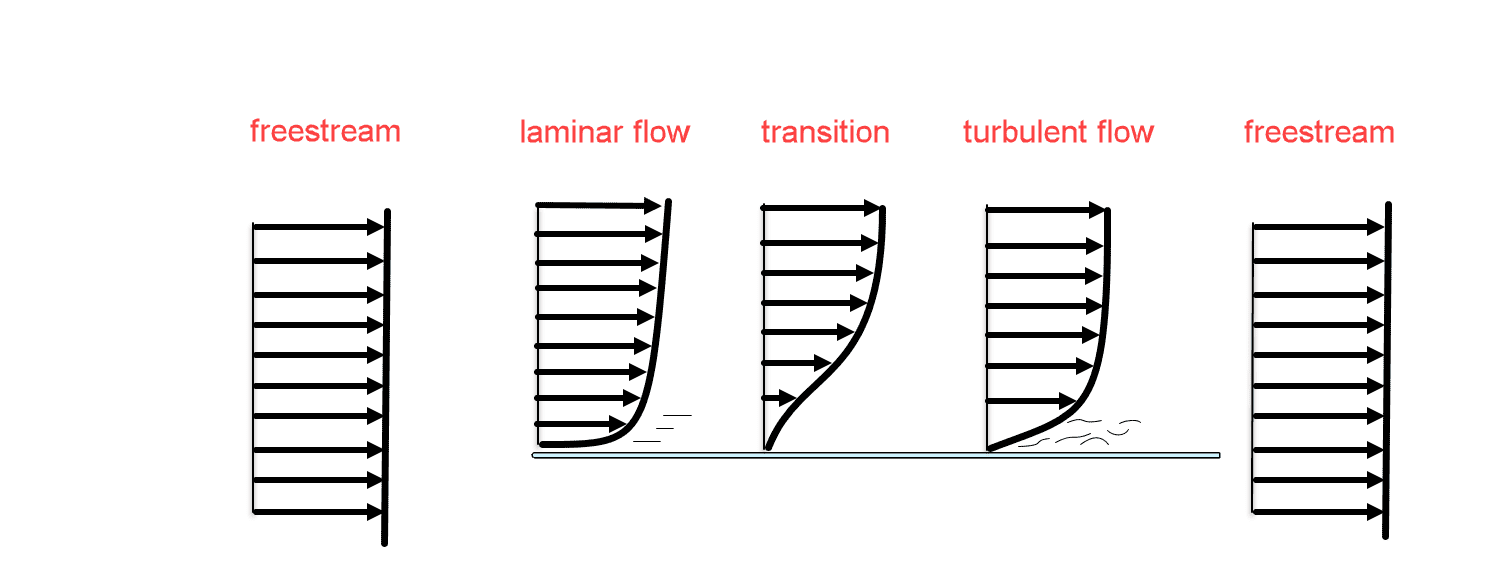
Laminar flow is considered as long as the fluid can stay attached to the surface. A laminar flow can be defined by the Reynolds number and a flat plate is considered when the Reynolds number is under 1800-2400. The Reynolds number is defined with $u$ as free stream velocity, $L$ as the length of the stream over the plate, and $\nu$ as the kinematic viscosity.

$$ Re := \frac{u*L}{\nu} \tag{1}$$

Turbulent Flow

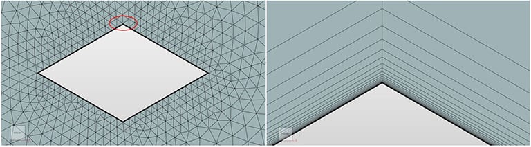
For higher Reynolds numbers the flow is considered turbulent. This means that the airflow is no longer able to stay attached to the wall and separates creating a turbulent boundary layer. To generate the boundary layer profile near the wall regions, two approaches are available.

Wall Function: Appropriate functions are used to model the velocity profile. Thus, the boundary layer profile is not completely calculated and a relatively coarse mesh can be used in the near-wall regions.

Note

To achieve a good accuracy with wall functions place the first cell of the mesh in the logarithmic region (30 < $y^+$ < 300).

Boundary-Layer Inflation of a Diamond Airfoil y+

What is y+?

Full Resolution: In this case, no functions are used and the flow profile is completely resolved. The mesh has to fulfill certain criteria and should be particularly of high resolution in the near-wall regions.

Note

For explicit resolution near the wall region, the first cell should lie in the laminar sub-layer region ($y^+$ < 1). Such a wall is referred to as fully resolved.

How to Choose Between Wall Resolution and Wall Modelling?

Types Of Wall Boundary Conditions And Which To Choose

There are four ways to define the flow velocity at the surface assigned with a Wall boundary condition within SimScale. These are:

No-Slip Boundary Condition

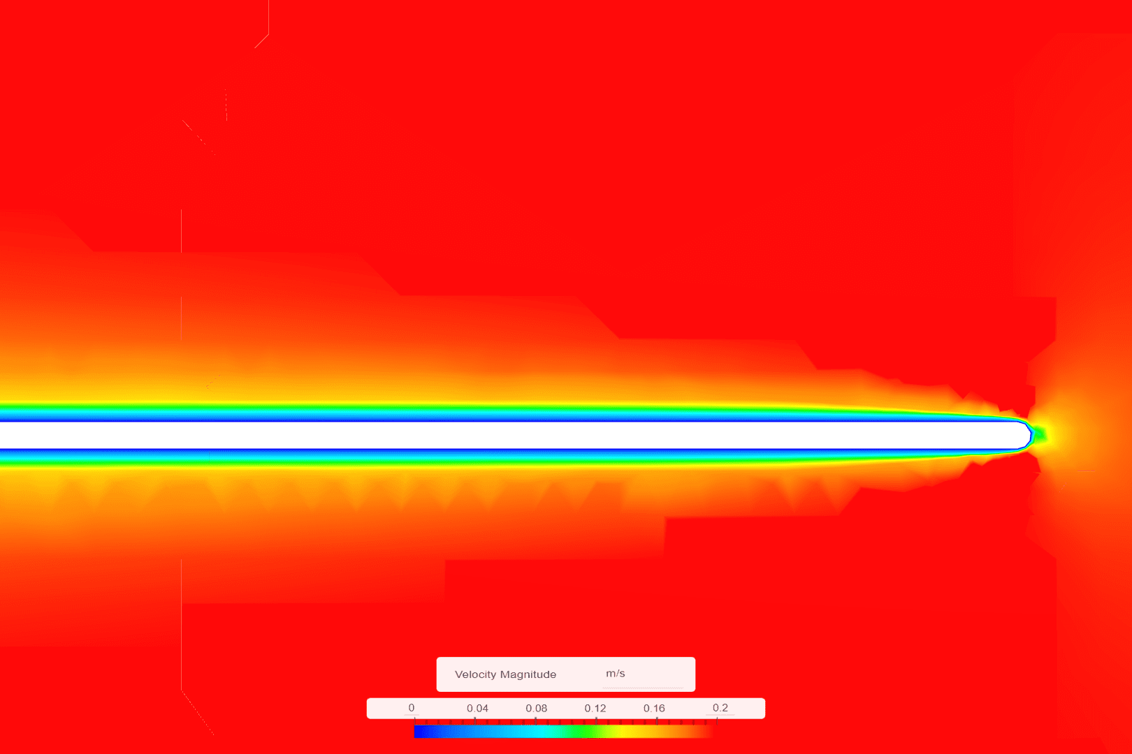
No-slip: Recommended for viscous flow and real-world surfaces with a velocity gradient from the wall to the freestream, with the velocity at the wall being zero.

Unassigned Surfaces

If any surfaces in the CAD model are left unassigned, then a No-slip wall boundary condition gets automatically assigned to them.

Some examples for No-Slip

Building facades with external flow
internal pipe surfaces with internal fluid flow
Airfoil surfaces with external flow

Wall Boundary Condition Wall_bopundary_no_slip_condition — Figure 2: No-slip condition for a free stream plate. With the No-Slip condition, the velocity gradient goes to a velocity of 0 $m/s$ at the surface of the plate.

Set Up For No-Slip Boundary Condition

Wall Boundary Condition Wall_Boundary_Conditio_Setup_NO-Slip — Figure 3: Setup for No-Slip Boundary Condition. Surfaces that are not assigned to a boundary condition are set as a No-Slip Wall

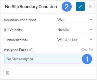
Since this is the default setting for wall boundary conditions only two changes have to be performed.

Assigned Faces: Assign face by direct selection or via a topological entity set.
Rename Boundary Condition: This is not mandatory, but it’s recommended as a best practice for a better overview of your project. All boundary conditions in SimScale supports this capability.

Slip Boundary Condition

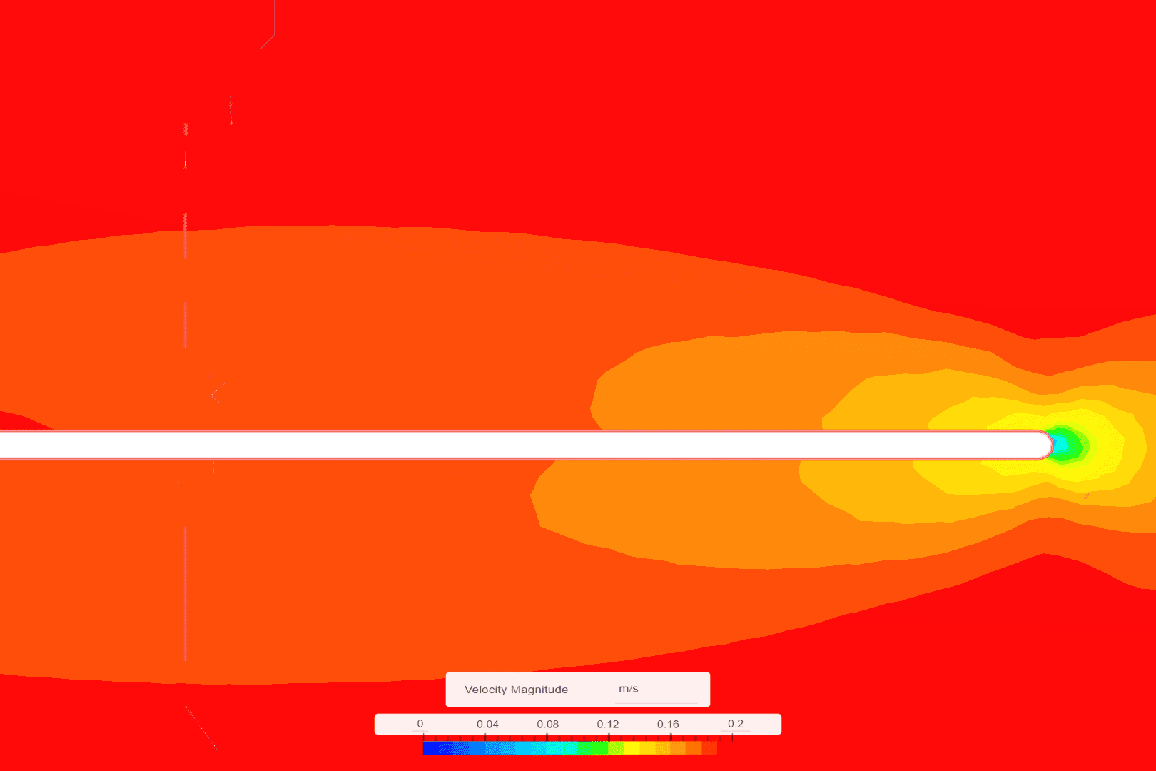
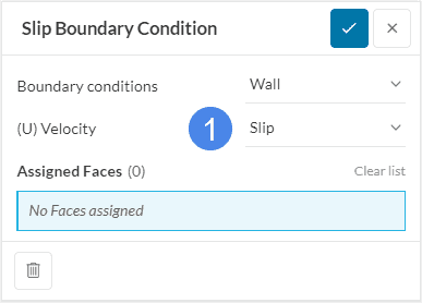
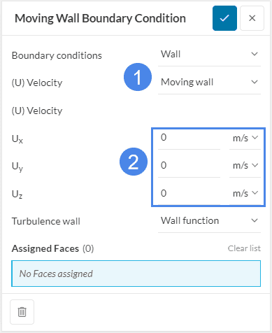
With Slip, a friction-less surface can be modeled. Mathematically speaking, it erases the normal component of the velocity and keeps the tangential components untouched at the assigned surface.

Example for slip boundary conditions

Simulation wind tunnel wall in external flow analysis

Wall Boundary Condition Wall_bopundary_slip_condition — Figure 4: Slip condition for a free stream plate. With the Slip condition, the velocity at the plate surface is the same as the free stream velocity, therefore there is no velocity gradient.

Set Up For Slip Wall Boundary Condition

Wall Boundary Condition Wall_Boundary_Conditio_Setup_Slip_2 — Figure 5: Set up for Slip Boundary Condition. Slip condition is mostly used for free stream walls of wind tunnels to reduce the effect of the wind tunnel on the simulation.

(U)Velocity (type): Switch the (U) Velocity type from No-Slip to Slip.

Moving Wall Boundary Condition

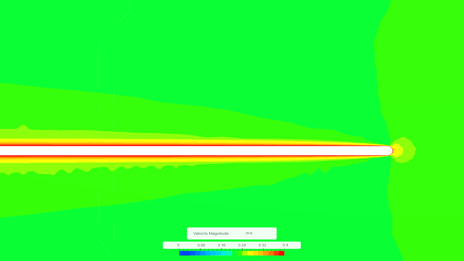
Moving wall boundary condition is used for a surface in motion. This means that the velocity gradient from the wall to the free stream velocity is not zero.

Some examples for Moving Wall boundary Conditions

Moving vehicle on the street or wind tunnel where the vehicle is modeled as stationary while the ground is in relative motion.
Belts running within a factory facility or in a wind tunnel

Wall Boundary Condition Wall_bopundary_moving_wall_condition — Figure 6: Moving wall condition for a free stream plate, with two times the free stream velocity at the surface.

Set Up For Moving Wall Boundary Condition

Wall Boundary Condition Wall_Boundary_Conditio_Setup_Moving_Wall_2 — Figure 7: Set up for moving wall boundary condition. Definition of the (U) Velocity vector is only appropriate for tangential flow

(U)Velocity (type): Switch the (U) Velocity type from No-Slip to Moving wall
(U)Velocity (Vector): Assign surface velocity as coordinates in the global coordinate system

Rotating Wall Boundary Condition

Rotating Wall: Used to specify the rotation of a wall surface about an axis. A point on the axis, the axis of rotation, and the angular velocity of the rotation must be specified. The latter could be specified as a constant, or as a time-dependent variable by either uploading a CSV file or directly entering the values in the table.
For general information on how to use the table feature in SimScale, refer to this document.

Some examples for Rotating wall boundary condition

Rotating tires of a car
rotating ball (sphere) through air

Wall Boundary Condition Wall_Boundary_Condition Rotating_Cylinder — Figure8: Rotating wall condition. Acceleration of the flow at the top of thy cylinder, deceleration at the bottom.

Set Up For Rotating Wall Boundary Condition

Wall Boundary Condition Wall_Boundary_Conditio_Setup_Rating_Wall_2 — Figure 9: Set up for rotating wall boundary condition. Rotating wall boundary conditions will only affect the surface velocity and cannot represent a rotating zone.

(U)Velocity (type): Switch the (U) Velocity type from No-Slip to Rotating Wall
Point on Axis: Define the center of rotation point within the global coordinate system
Rotation Axis: Define the rotation axis in the global coordinate system.
Rotational Velocity: Define the angular velocity of the surface either via direct input or for transient simulations define or import a table. You can also change the Unit of the rotation from $rad/s$ to $°/s$

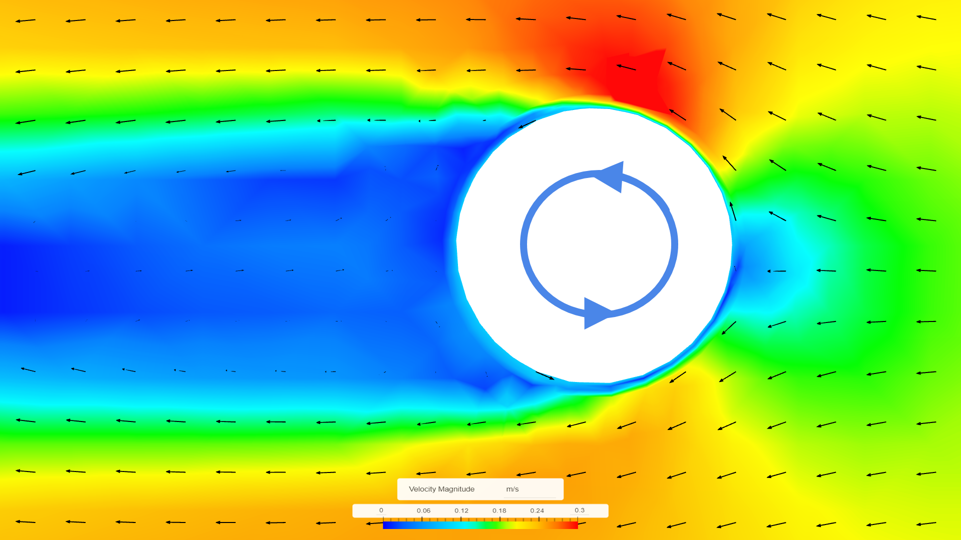
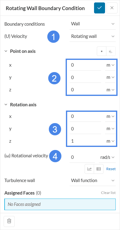
Direction of rotation

When defining the rotation axis, or the Rotational velocity ,please follow the right hand rule for positive rotation directions.

How To Choose Between Rotating Zone and Rotating Wall?

External Vehicle Aerodynamics
External Building Analysis
Internal Pipe Flow (Note the use of the default assignment on not assigned boundary faces)

Example

The best example to understand the different wall types is that of a moving car. For simulation, the car is stationary and the air is blown at it through the inlet face (red).

Wall Boundary Condition Car_reference_wall_boundary_conditions_2 — Figure 10: Example of a moving car domain ready for CFD simulation. The four different wall boundary conditions are shown.

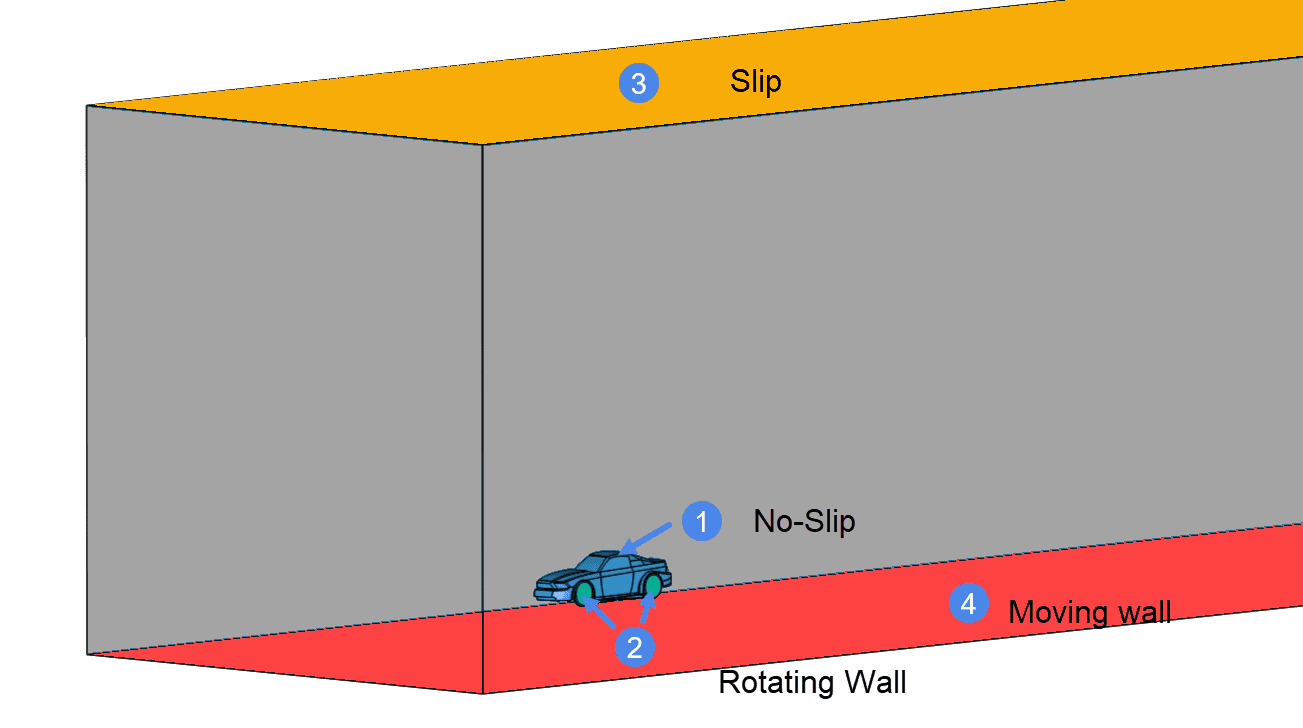
Here, car body (1) is assigned no-slip, tires (2) are rotating walls, ground (4) is a moving wall (since no relative motion between air and ground), and the top along with the outer face (3) is defined as a slip wall condition.

Slip v/s Moving Wall Condition for Street Simulation

When in reality, the car moves through the air, the air is not moving relative to the street. Therefore there is no boundary layer between the air and the ground. To take this into account the ground in the simulation should be assigned a condition which doesn’t create a boundary layer. For this either the Slip or the Freestream boundary can be selected.

However, for some cars the undertray or wings are too close to the street because of which the the air velocity underneath the car can differ from the free stream velocity. This results in a speed difference that can create a boundary layer for the air underneath the car and the street. To take this into consideration a Moving wall boundary condition is used. This makes sure that the free stream air doesn’t have any boundary layer, but for regions where the airspeed is different from the free stream speed a boundary layer can still be resolved.

Thermal Boundary Layer

For simulation which considers temperature gradients or heat sources, the thermal behavior of the wall has to be defined.

All details about the available choices and their implementation are described in the following knowledge base articles:

Without radiation

How to Set the Right Thermal Wall Conditions in CHT Without Using Radiation?

With radiation

How to Assign Wall and Window Settings for Thermal Comfort Simulations?