Tutorial: Fluid Flow Through a Non-Return Valve

This article provides a step-by-step tutorial for a fluid dynamic simulation of a non-return valve.

Overview

Valves under particular flow conditions can be simulated to obtain key performance quantities such as pressure drop through the system. Additionally, velocity and pressure results can be inspected in detail to identify regions of extreme pressure and flow inefficiencies. This tutorial acts as a guide for valve analysis best practices and can be used as a template for your future projects.

We are following the typical SimScale workflow:

1. Preparing the CAD model for the simulation.
2. Setting up the simulation.
3. Creating the mesh.
4. Run the simulation and analyze the results.

1. Prepare the CAD Model and Select the Analysis Type

First of all, click the button below. It will copy the tutorial project containing the geometry into your Workbench.

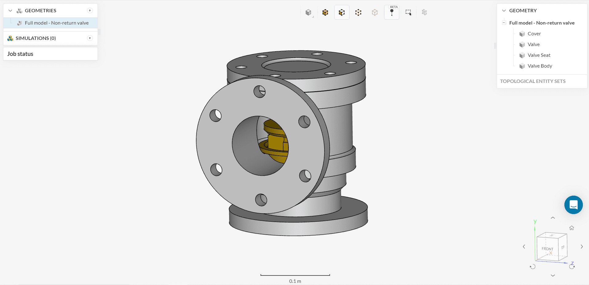
The following picture demonstrates what should be visible after importing the tutorial project.

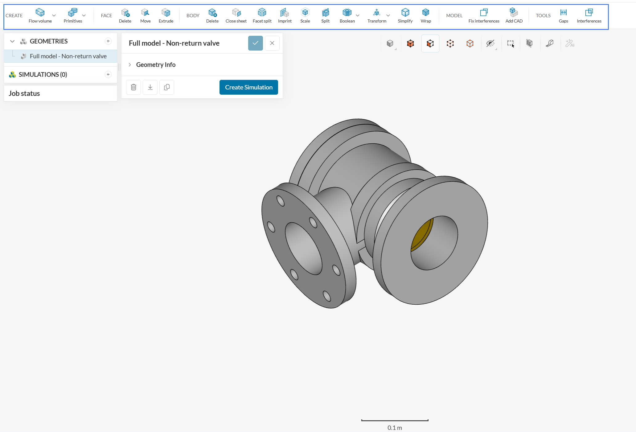
1.1 Editing the CAD Model

The initial geometry contains an assembly with the components of the valve. Before we can begin a flow simulation, first we have to create the fluid volume. To do this, we are going to use the CAD edit functionality:

In this stage, we have three main objectives:

• Create an Internal Flow Volume
• Delete the solid components of the valve
• Optimize the flow region geometry for simulation

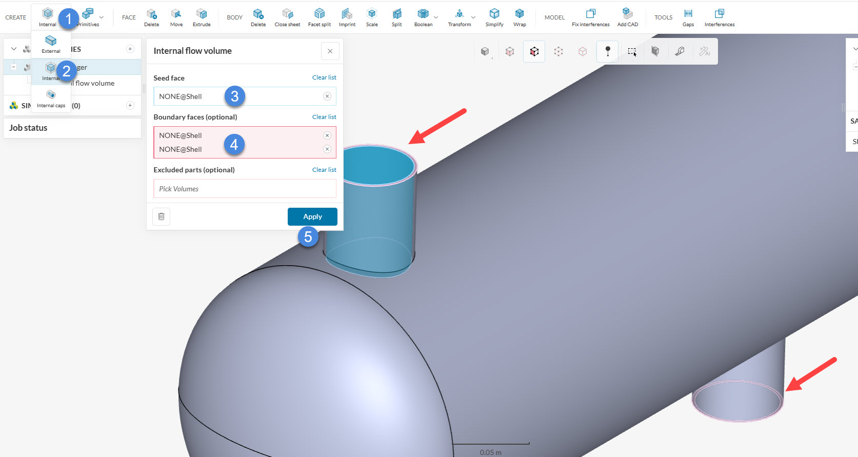
The first objective requires an Internal Flow Region operation, which is performed through the steps shown below:

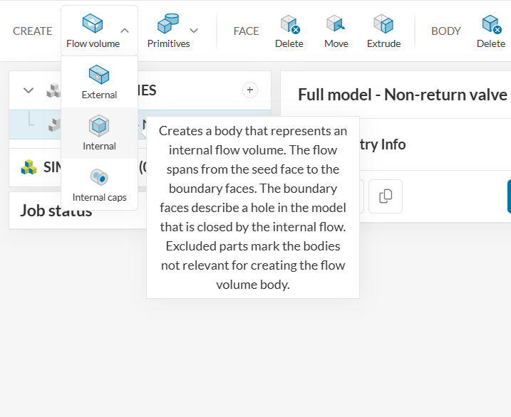
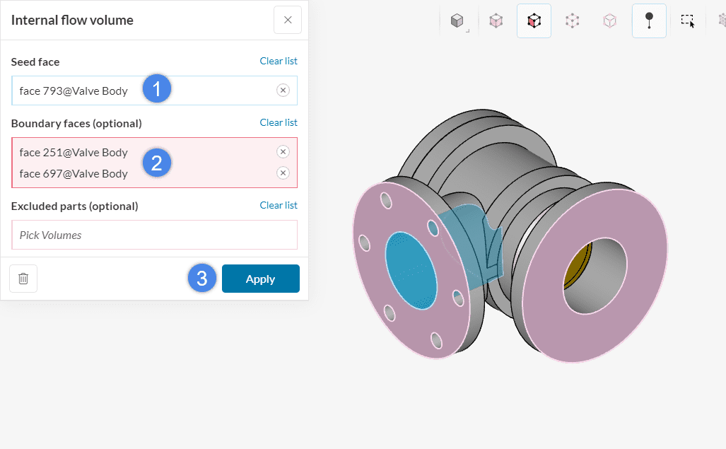
1. Select the ‘Create – Flow volume – Internal’ operation.
2. Select a Seed face, which can be any internal face that will be in contact with the flow region. In Figure 4b, the selected seed face is highlighted in light blue, corresponding to the internal face of the outlet nozzle.
3. Define Boundary faces of the geometry. These faces contain the openings of the flow region. In our case, we have the two boundaries highlighted in white in Figure 4b, corresponding to the flanges end faces. In case you are in doubt about the boundary faces of your geometry, consider visiting this page.
4. Hit ‘Apply’ to run the operation.

After the operation runs, you will notice that we have one additional volume: the Flow region. For single-region analysis types, such as incompressible, this is the only volume that we need to run the simulation. Now, our goal is to delete the components of the valve with a Delete Body operation:

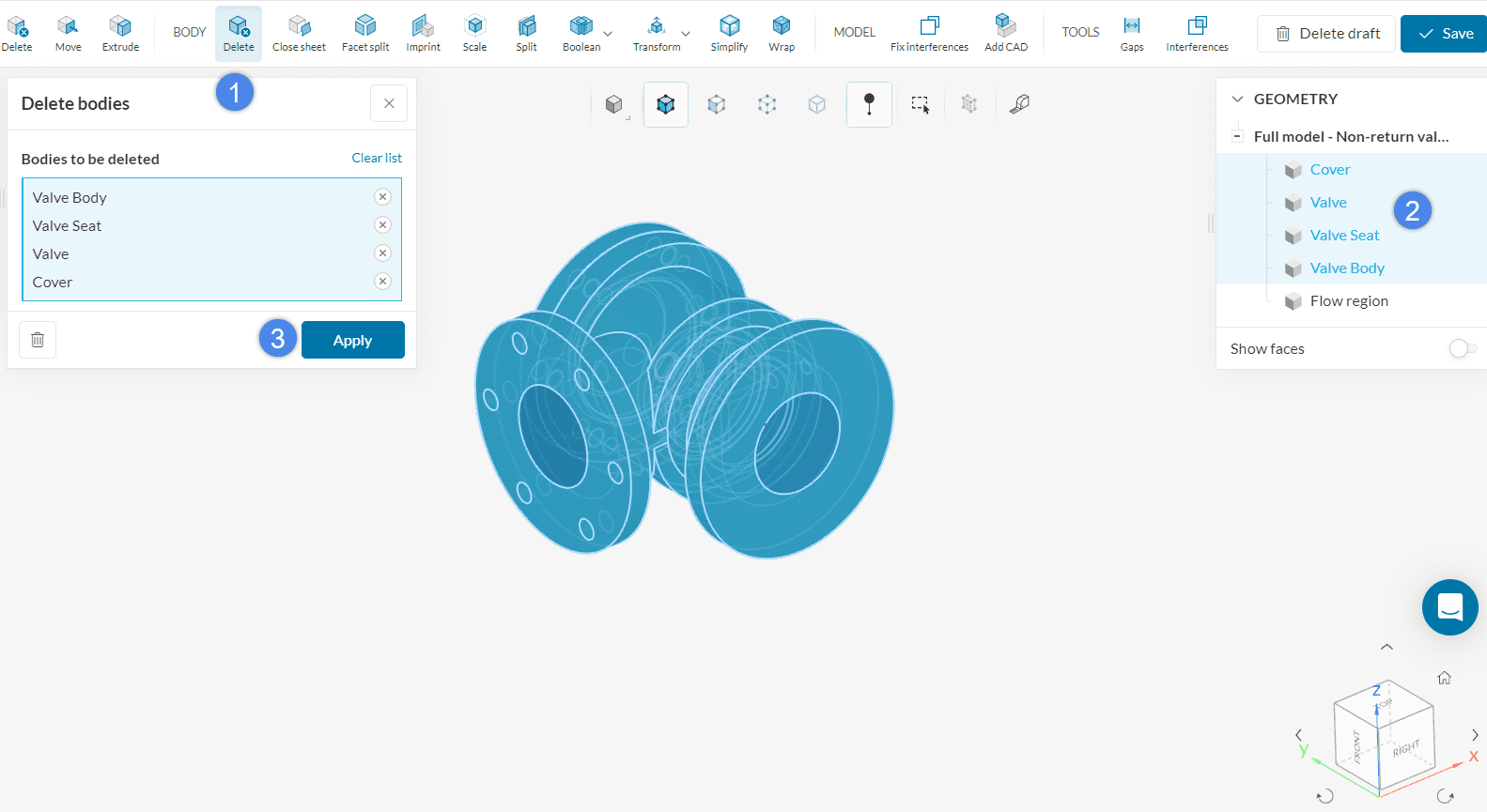
1. Create a ‘Body – Delete’ operation.
2. Select the valve components from the GEOMETRY panel on the right-hand side.
3. Hit ‘Apply’.

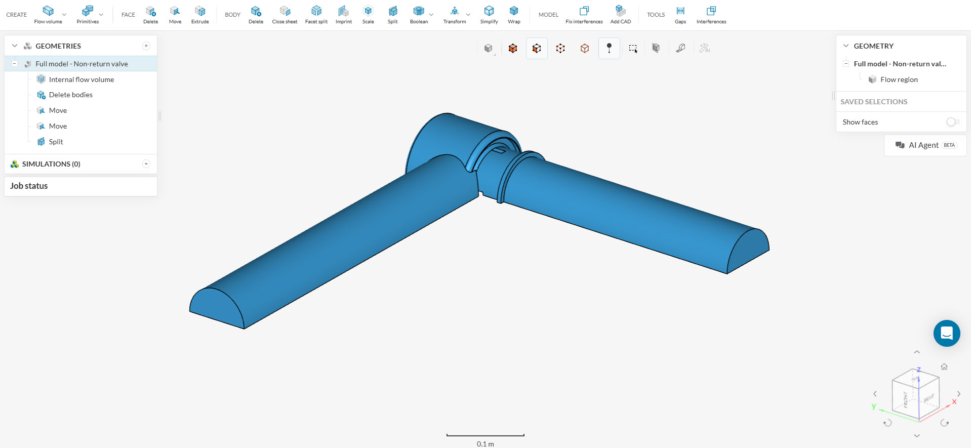
After the operation completes, we can see the flow region geometry without the solid components. Our next goal is to optimize this geometry for simulation, which will be achieved by:

• Extending the inlet and outlet faces to stabilize the flow.
• Cutting the geometry in half to leverage the symmetry and saving on computational resources.

To extend the inlet face, we make use of the Move Face operation:

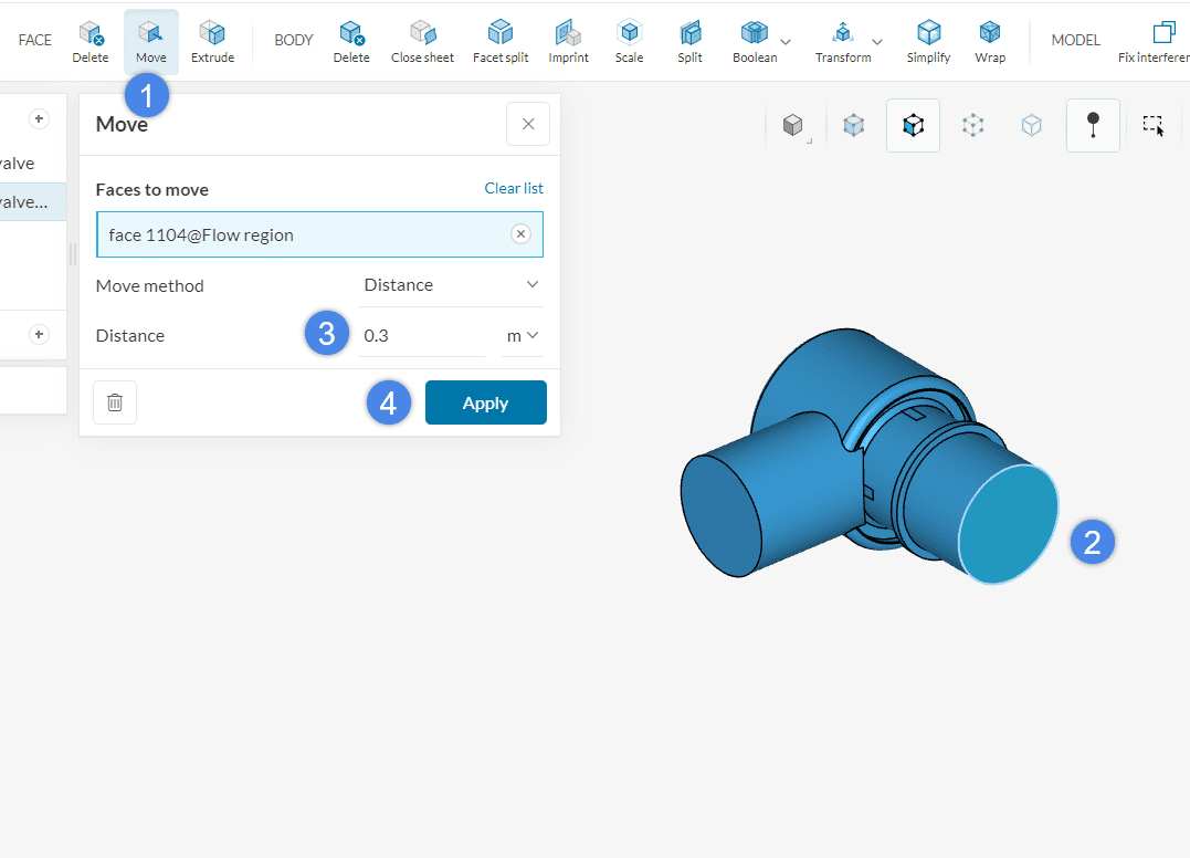
1. Create a ‘Face – Move’ operation
2. Select the inlet face for Faces to move
3. Input a Distance of 0.3 \(m\).
4. Click ‘Apply’ to perform the operation

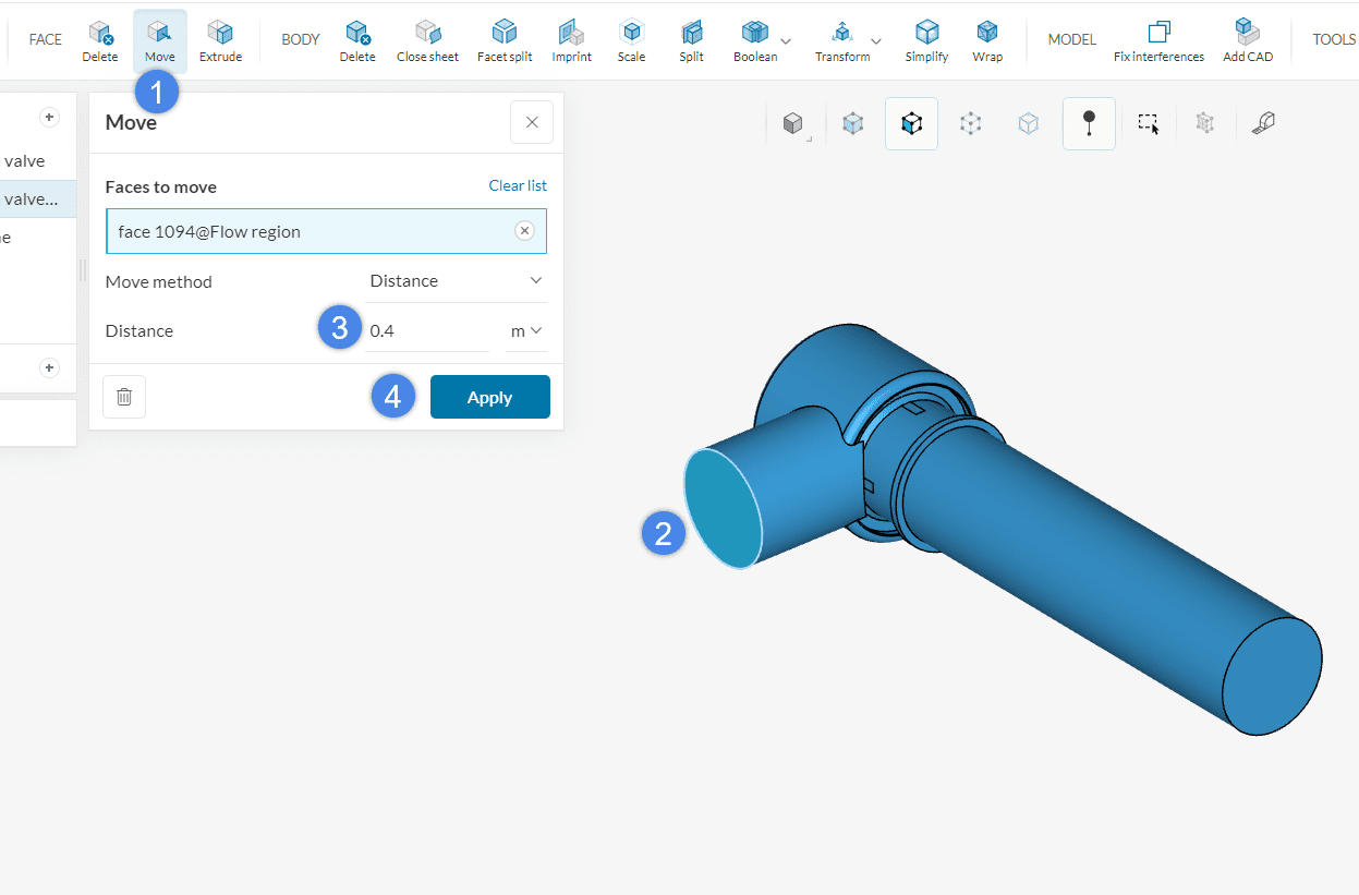
Now we repeat the steps on the outlet face, this time extending it by 0.4 \(m\):

Finally, to cut the flow region in half and leverage the symmetry, we use a Split operation:

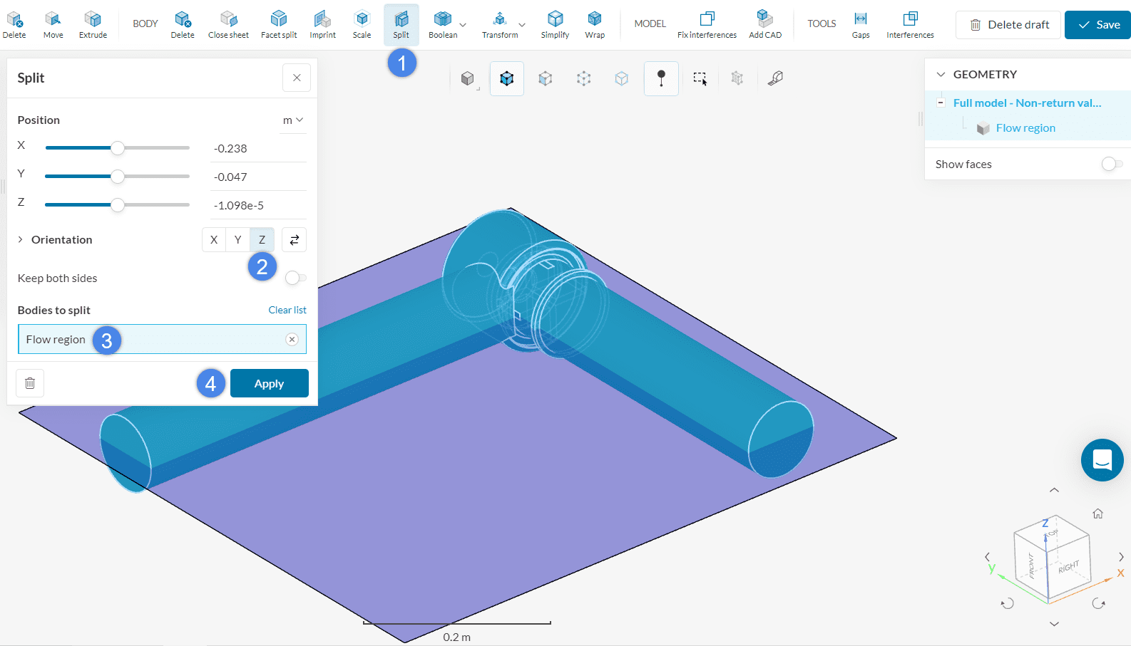
1. Create a ‘Model – Split’ operation.
2. Select the ‘Orientation – Z’, because the model is symmetric around the XY plane, which is normal to the Z axis. The Inverse button allows you to select which side of the plane will be kept.
3. Assign the operation to the ‘Flow region’ volume
4. Click ‘Apply’ to perform the operation.

For the tutorial we use the half that is in the Z-direction. After you have done it, click the ‘Save as copy’ button at the top right:

1.2 Create a Simulation

After saving the draft, you will see a second geometry in the GEOMETRIES tab. This is the one that we are going to use to run the simulation. We can change the name of the new model to something more representative before creating a new simulation. Therefore, please proceed as below:

1. Change the name of the new CAD model to Non-return valve – Flow region.
2. Click on the ‘Check’ icon to save.
3. Click again on the geometry Non-return valve – Flow region and now we are ready to click on ‘Create Simulation’. Alternatively, click on the ‘+‘ icon next to Simulations to create a simulation.

At this point, the analysis type selection widget opens up:

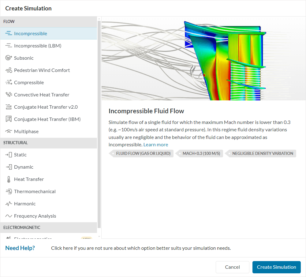
In this simulation, we calculate the flow of water through a valve. As long as the speed of the fluid is subsonic (Mach Number below 0.3), we select the incompressible analysis and create the simulation.

2. Assign Materials and Boundary Conditions

2.1 Define a Material

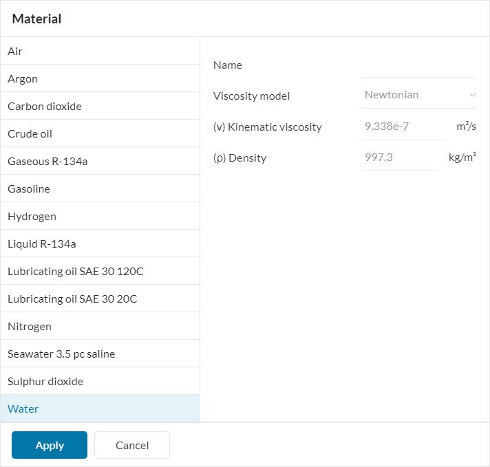
To apply the material to the geometry, press the ‘+ button‘ next to Materials to open a list with options. For this simulation, we will select ‘Water‘ and press ‘Apply‘ to confirm the selection.

Since we have a single volume, the material is automatically assigned to our flow region. Therefore, we can proceed to the boundary condition set up.

2.2 Assign Boundary Conditions

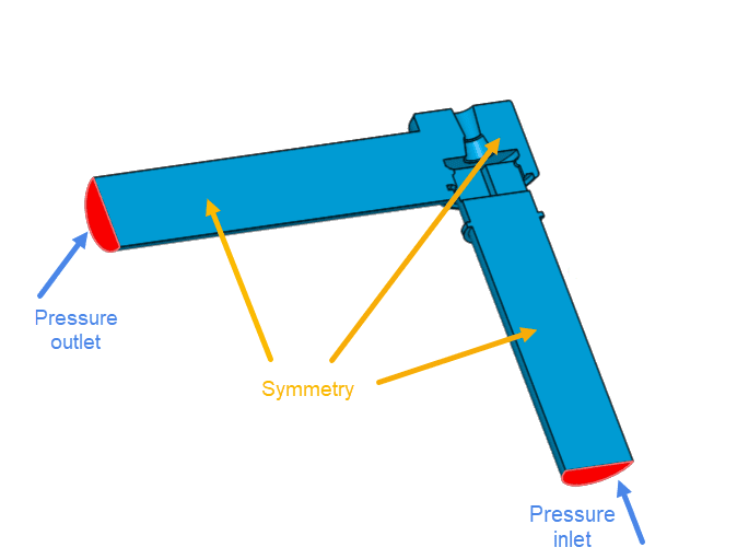
In the next step, boundary conditions need to be assigned. Here, the goal is to define the physics of the simulation, including inlet, outlet, symmetry plane, and physical walls.

To have an overview, the following picture shows the boundary conditions applied for this simulation:

a. Flow Conditions

Starting with the flow conditions, one needs to assign a Pressure inlet condition to the inlet as shown below:

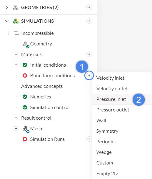
After hitting the ‘+ button’ next to boundary conditions there will pop up a drop-down menu where one can choose between different boundary conditions.

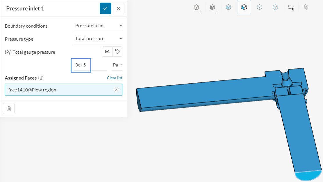
Assign a Pressure inlet condition with a total gauge pressure of 3e+5 \(Pa\):

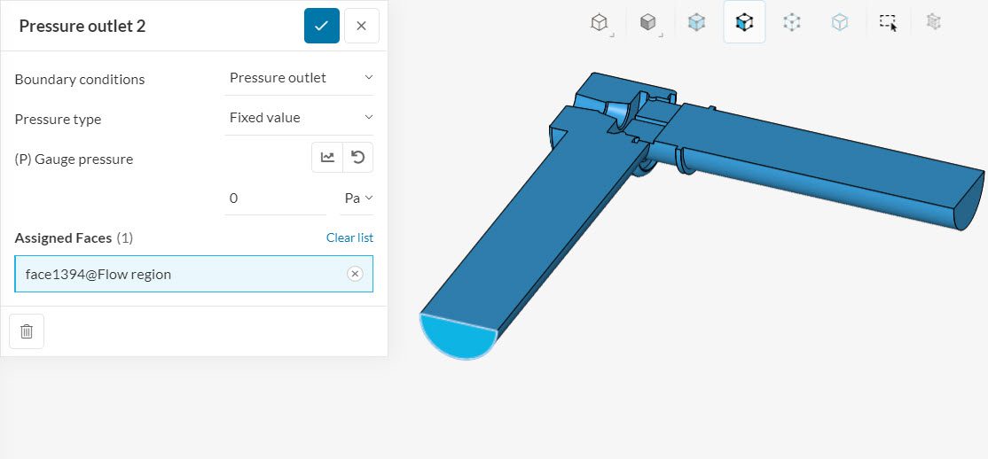
Lastly, we will assign a Pressure outlet condition with a fixed value of 0 gauge pressure to the outlet. This sets the outlet to atmospheric pressure allowing flow to exit freely.

To create a pressure outlet boundary condition, you can follow the same steps from Figure 13.

From the flow standpoint, these are the only two boundary conditions necessary. We can now define the symmetry condition for the geometry.

b. Geometry Conditions

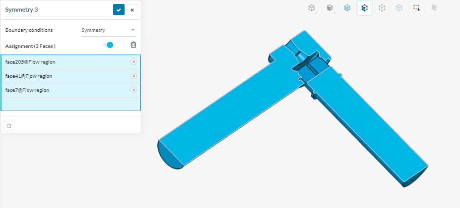
Now we will assign symmetry conditions to all the surfaces that lie directly on the plane of symmetry. To do this, create a new boundary condition type Symmetry, and select the three surfaces.

2.3 Simulation Control and Result Control

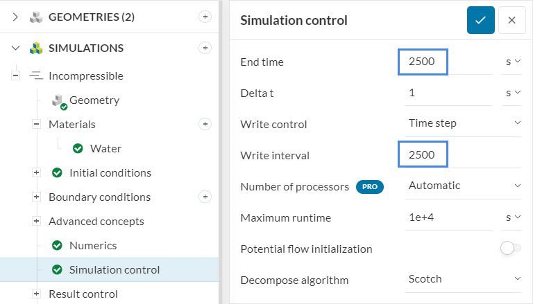
Please navigate to Simulation Control in the simulation tree. The Simulation control tab allows you to change several settings, including the number of iterations and maximum runtime for the simulation.

For this tutorial, we are going to change both End Time and Write Interval to ‘2500’. With these settings, we will run a total of 2500 iterations and write only the final result set.

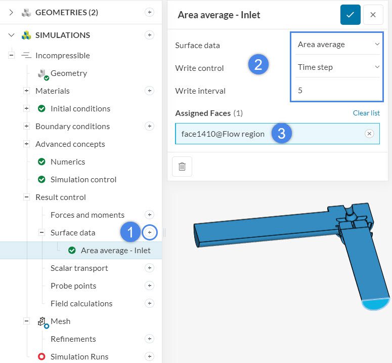
You can also use Result controls to observe the convergence behavior of certain items of interest. In this simulation, let’s keep track of the inlet values by setting an Area average result control. Please follow the steps below:

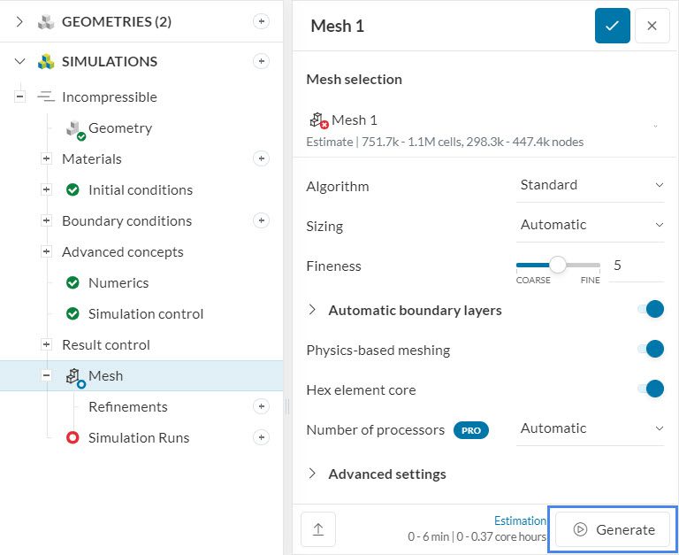
3. Mesh

To generate the mesh, we recommend using the Standard algorithm, which is a good choice in general because it is quite automated and delivers good results for most geometries.

For this initial analysis, we are going to create a standard mesh with default settings. Therefore, simply click on ‘Generate’ within the mesh setup window.

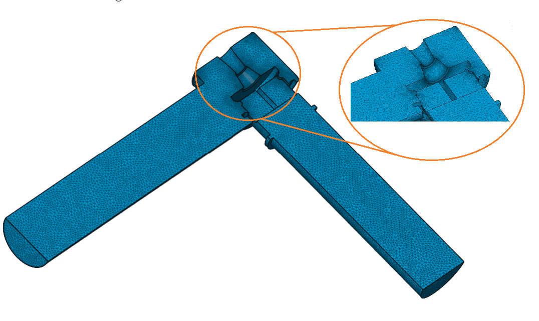
After a few minutes, the mesh finishes running and will have the following aspect:

4. Start the Simulation

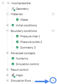
Now you can ‘Start’ the simulation, and after 1 to 2 hours, you can have a look at the results.

5. Post-Processing

Once your simulation run is complete you can use the online post-processor to visualize the results. To become more familiar with the post-processor, please refer to the following documentation.

Before jumping into the post-processor, it’s a good practice to evaluate the convergence of the simulation. The result controls are very valuable for this purpose. For example, let’s check if the velocity is stable at the inlet of the system, by inspecting the Uy-component:

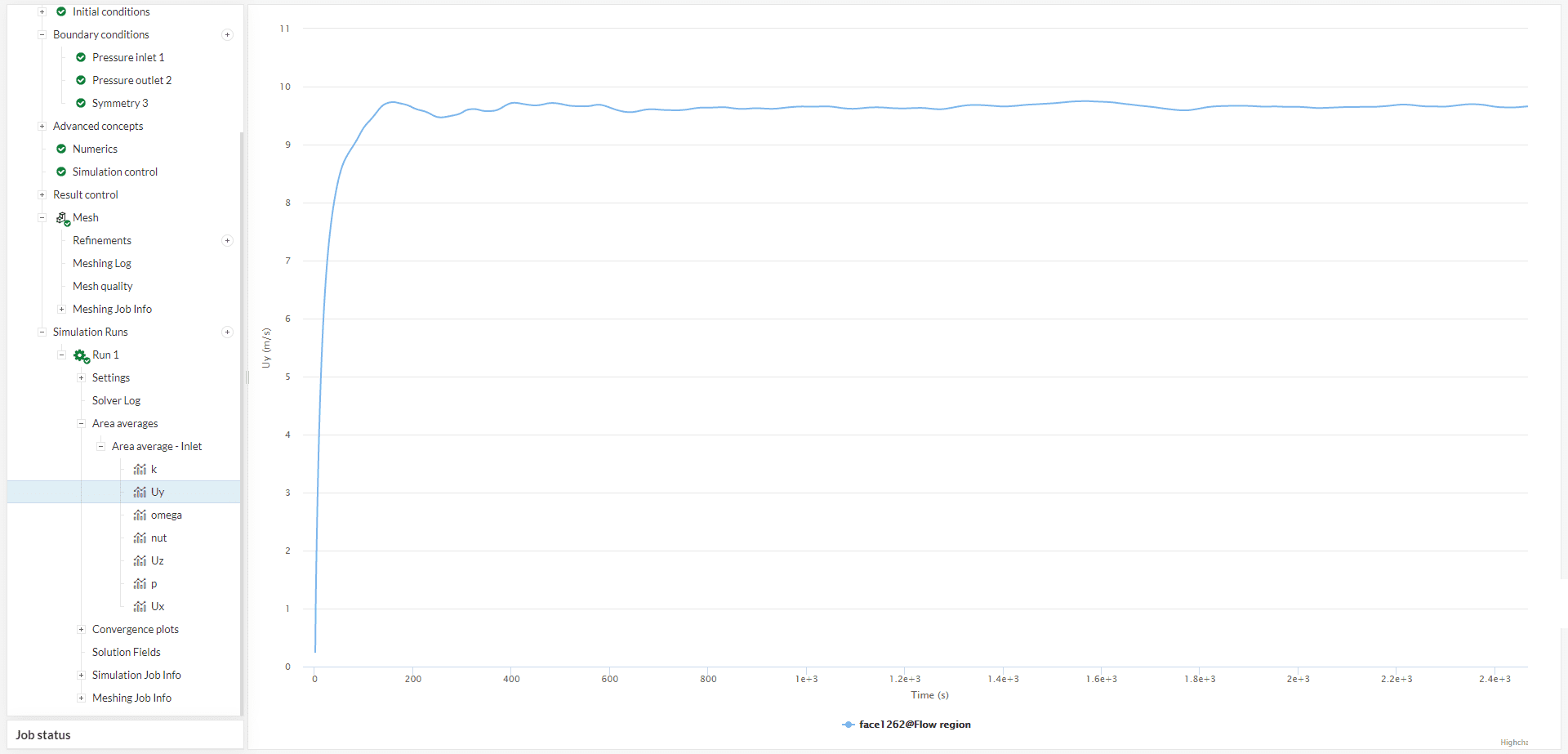
When analyzing valves, it is interesting to calculate the pressure drop and observe the velocity behavior through the system and whether any backflow occurs. Open the online post-processor by selecting ‘Solution Fields’ under the completed simulation run.

a. Pressure Drop

The pressure drop across the valve is computed by using the result statistics calculator. Here are the steps:

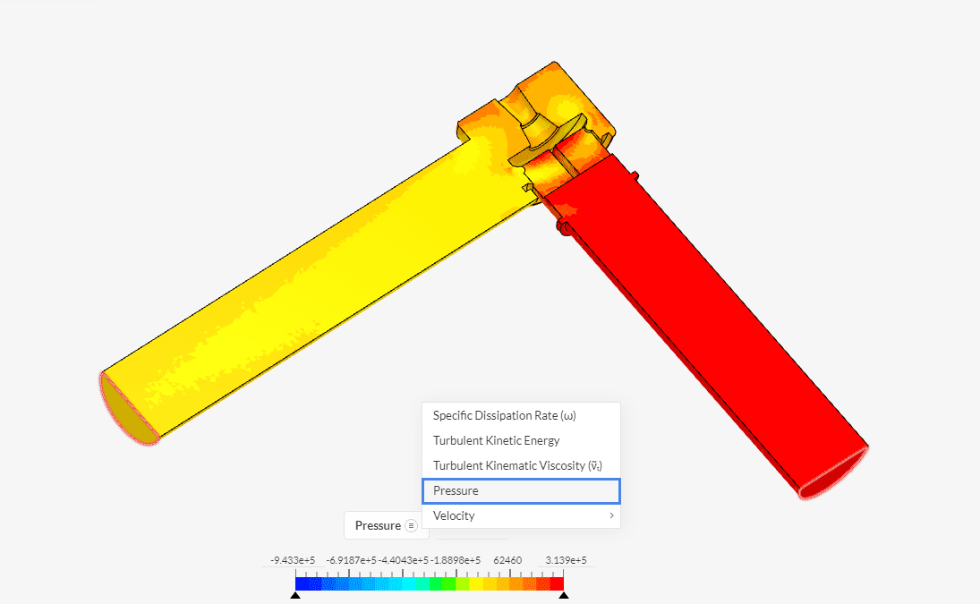
First, select the Pressure field for coloring (and statistics) of the model:

Make sure that there is no Cutting Plane filter applied in the model. If there is any, remove them by using the trash-can icon.

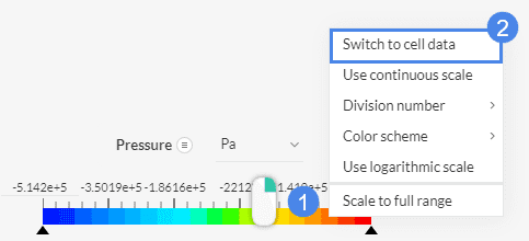
Whenever using the statistics calculator, it’s recommended to switch the data set to cell data. To do that, you can right-click on the legend and select ‘Switch to cell data’ from the drop-down menu. The image below illustrates the process:

Now we are ready to toggle on the Statistics calculator. Select the ‘View – Statistics’ item from the top bar. A panel containing the statistical information will appear on the top right corner of the viewer.

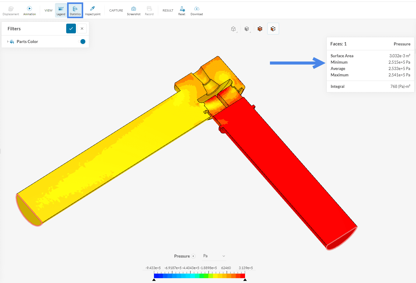
Now you can select the inlet face of the model, and find that the average pressure is 2.533e+5 \(Pa\). If you unselect the inlet face and then select the outlet face, you should see an average pressure of 0 \(Pa\), which is the value imposed in our boundary condition. Therefore, the total pressure drop across the valve is 2.533e+5 \(Pa\).

You can also find more ways to calculate the pressure drop with flow simulations here.

b. Backflows

Backflow is another phenomenon that is important when evaluating a valve. We will visualize the flow on a cutting plane of the valve with the following steps:

1. Create a ‘Filter – Cutting plane’ from the top bar.
2. Change the orientation to (normal to) ‘X’ axis.
3. Change the position of the cutting plane to the following coordinates: (0.02, -0.022, -0.032). You need to expand the Position dropdownto access the coordinate input. This will center the cutting plane on the inlet pipe.
4. Enable the ‘Vectors’ visualization. Set the Scale factor to ‘0.02’ and the Grid spacing to ‘7.5e-3’.
5. To improve the visibility of the vectors, change the Coloring to ‘Solid color’, and select a dark gray or black color from the picker.
6. Also, enable ‘Project vectors onto plane’.

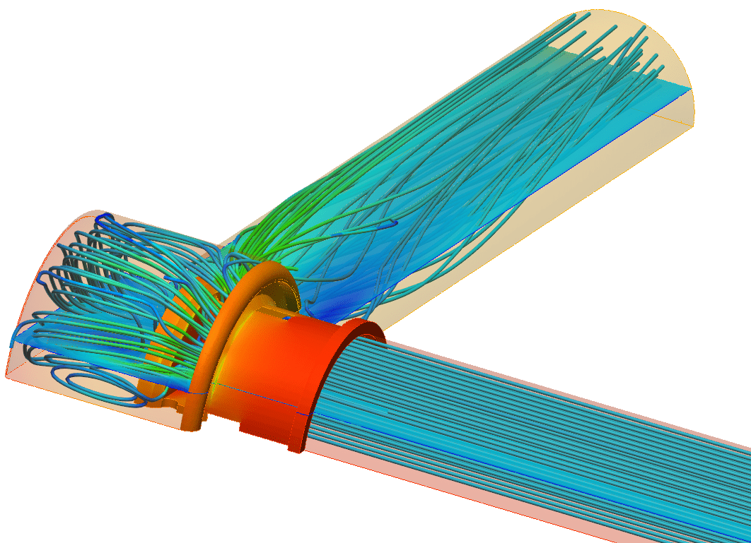
You should get a visualization similar to this:

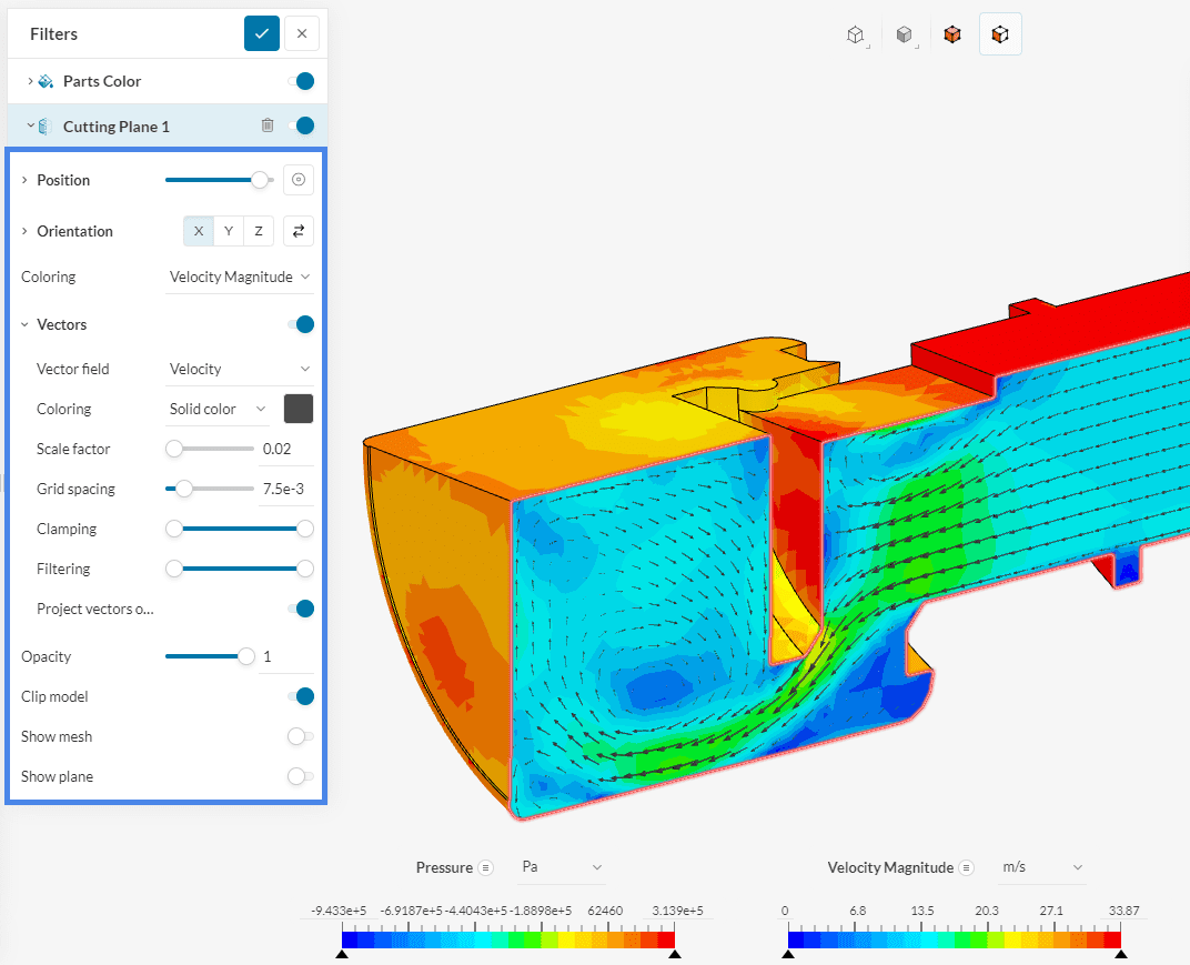
We can see from the figure above that there is backflow occurring near the entrance of the valve and there are swirls inside of the valve cavity. This could impact the valve performance as it hinders the flow patterns at critical locations, increasing the pressure drop.

Analyze your results with the SimScale post-processor. Have a look at our post-processing guide to learn how to use the post-processor.

Congratulations! You finished the tutorial!

Last updated: October 29th, 2024