Tables

By using a table input, users can specify a variable (velocity, temperature, etc) along with another independent variable (e.g time or distance).

Not every variable is allowed to be defined as a function of another variable. If tables are allowed, you can find the icon of a graph next to the variable you want to define.

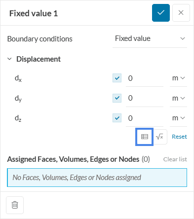
using tables feature simscale — Figure 1: Boundary conditions can be defined using tables when the highlighted icon is available.

Once you click on the icon, a dialogue box appears to define the table. The example below shows a table input for a time-dependent temperature boundary condition. The data can be uploaded in CSV format or dynamically manipulated at the interface.

general table interface — Figure 2: Table for time-dependent temperature boundary condition. Here t is time in seconds and *Value* represents temperature in kelvins.

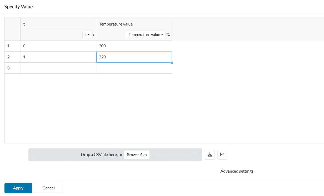
The CSV file should just contain the input values (no title, index numbers, etc.). Every line in the text file will define a row and values separated by a comma ‘,’ will define the columns. As an easy example, the CSV file for the table seen above should be like the following:

0,300
1,320

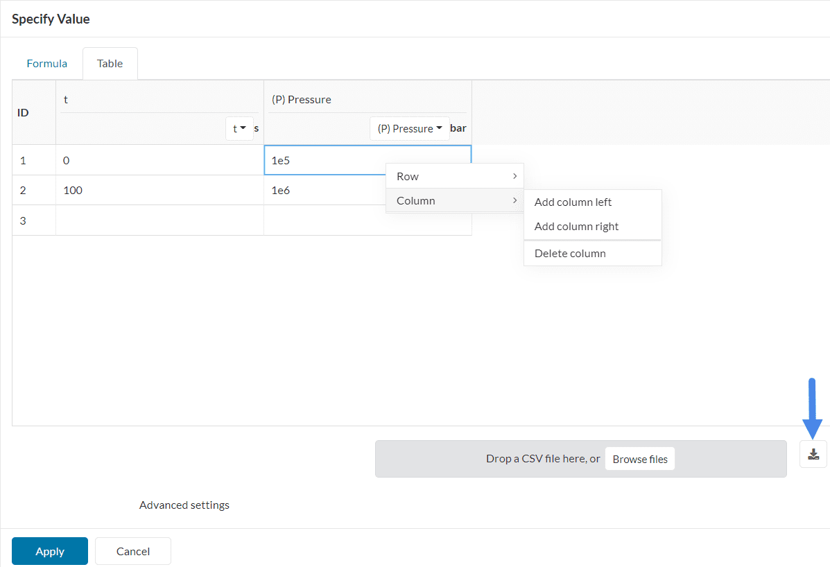
Once the CSV file is uploaded, the variable for each column should be properly set. Values can be manually modified and rows/columns can be added/deleted by right-clicking on any cell. The data from the table can always be downloaded by pressing the icon next to ‘Browse files’.

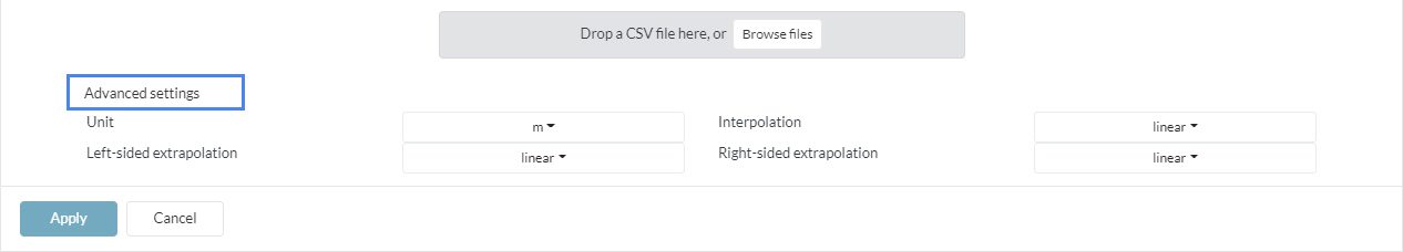
adding or deleting rows and columns table input — Figure 3: By right-clicking on a field, you can add/delete rows and columns. The blue arrow points to the download button.

Advanced Settings

For CFD analysis types, after clicking on Advanced settings, two options appear:

Units: It is possible to define different units for some variables such as temperature or distance.
Out of bounds: By default, it is set as ‘Use nearest‘. It means that the regions out of the defined range in the table are defined by the nearest value. Hence, the last value in a given coordinate will be kept constant till the end of the domain.

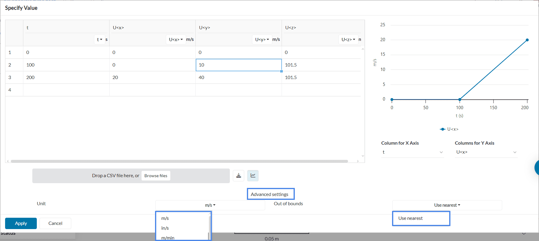
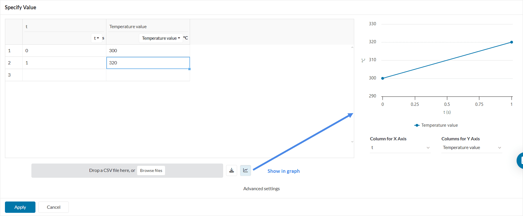
expanding advanced settings table definition — Figure 4: To open the advanced settings, you can click on the highlighted button at the bottom of the table window.

As an additional note, the interpolation between two points in CFD is always linear. A visual representation of the table input from Figure 4 is shown below:

velocity definition cfd table input — Figure 5: In CFD, the interpolation between points is linear, and the nearest value is used when out of bounds.

Important

For Code_Aster-based solvers you can as well specify the interpolation and the extrapolation type between the given value pairs:

advanced settings tables code aster — Figure 6: Advanced settings for Code Aster based solvers in SimScale allow specifying units, the type and interpolation, and extrapolation.

Examples 1: Variable Vector

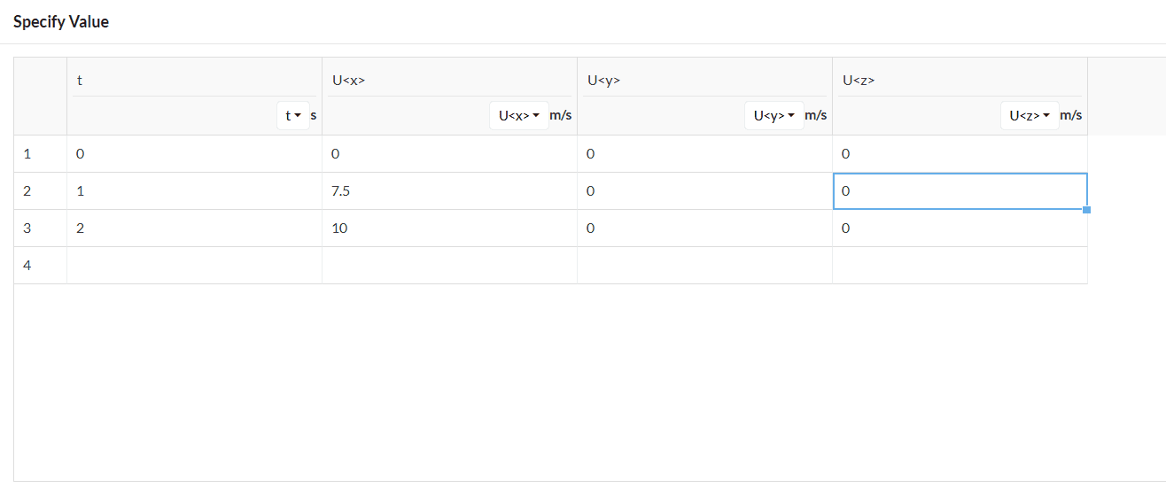
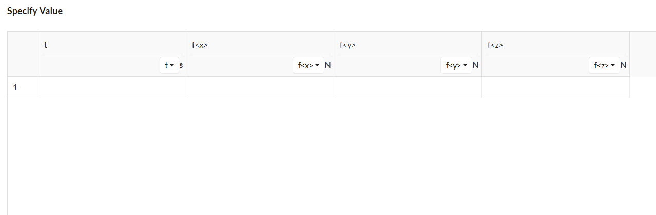
For ‘Vector’ variables (e.g velocity) the table upload requires a CSV file with the independent variable and all 3 velocity components in the order X, Y, and Z for each point. Depending on the independent variable we can find two different types of tables:

Time distribution: Velocity is assigned for every time instant defined in the table. Over time, a uniform velocity on the assigned faces is defined. A 4-column CSV file can be uploaded with time and velocity values (t,Ux,Uy,Uz).

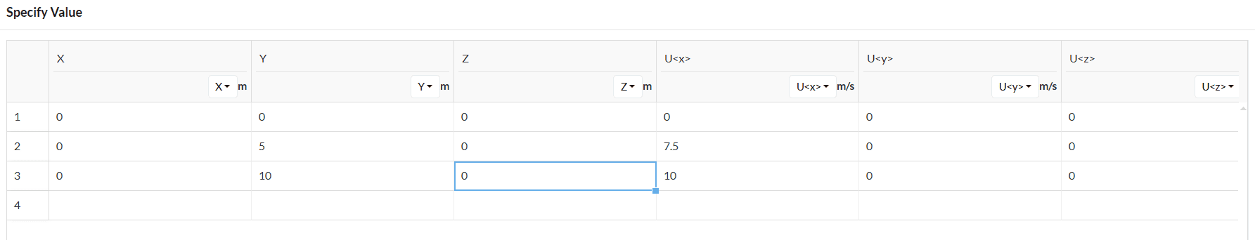
table for velocity components along time — Figure 7: Time-dependent velocity table. Three velocity components are defined for every desired instant of time.

Spatial distribution: Velocity is defined for every spatial coordinate of the assigned boundary condition face. In the figure below, a velocity profile in the x-direction has been defined based on the x, y, and z coordinates. A 6-column CSV file can be uploaded with time and velocity values (x,y,z,ux,uy,uz).

Velocity components tables simscale — Figure 8: Space-dependent velocity table. Three velocity components are defined for every component of space in the desired location.

Example 2: Variable Maximum Time Step Length for FEA

For nonlinear FEA studies, such as dynamic and nonlinear static, the user can define different Maximum time step lengths throughout the simulation under the Simulation Control settings.

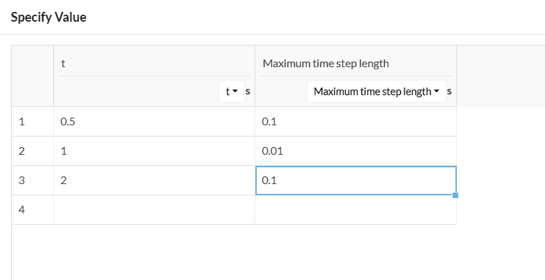
maximum time step length definition nonlinear FEA — Figure 9: Variable maximum time step length definition for nonlinear static and dynamic simulations

With the definition above, the following result is obtained:

From t = 0 until t = 0.5 s: timesteps of 0.1 s each
From t = 0.5 until t = 1 s: timesteps of 0.01 s each
From t = 1 until t = 2 s: timesteps of 0.1 s each

Note for Nonlinear FEA Studies

For nonlinear finite element analyses, the t = 0 timestep is never solved, since it is controlled by the initial conditions defined by the user. Therefore, boundary conditions defined via table definition will not be considered for the t = 0 step.

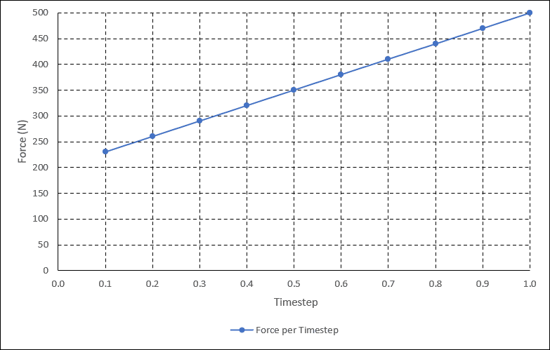
As an example, consider a dynamic study with a timestep size of 0.1 seconds where the user defines a force boundary condition with the table below:

Figure 10: Force boundary condition definition for a dynamic study. In this example, the interpolation is linear between steps.

For the time = 0 step, the 200 Newtons definition will be ignored, since the initial conditions will control the results.

Considering a linear interpolation, from the first timestep onwards the force will increase by 30 Newtons per step. The graph below shows a visual representation:

table definition timestep 0 nonlinear fea simulations — Figure 11: Force that is applied during a nonlinear FEA study per timestep

Try it Yourself

The following are some of our tutorials where you can try using the tables feature:

Last updated: July 19th, 2022

Did this article solve your issue?

How can we do better?

We appreciate and value your feedback.