How to Assign Wall and Window Settings for Thermal Comfort Simulations?

The objective of this article is to show how to set boundary conditions for walls and windows in thermal comfort (convective heat transfer) simulations.

Walls

Walls in reality are composed of multiple layers of different materials, such as concrete, brick, insulation, paint, etc. In thermal comfort simulations, we are only interested in the temperature of the air domain and use some simplifications to imitate heat transfer between the walls of the domain with external conditions.
Solid surfaces are treated with ‘Wall‘ boundary conditions. As a default, every surface, which has no boundary condition is treated as an adiabatic wall. In the following section, you will see the settings for some common wall conditions.

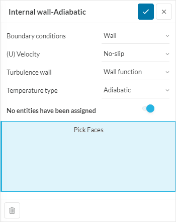
Adiabatic Wall

An adiabatic wall means that there should not be any heat transfer between the surface (surface of the fluid domain) and the surroundings. Usually, internal walls are assumed to be adiabatic, since the same temperature conditions are expected in the neighboring rooms.
As a rule of thumb, one can use laminar flow for natural convection, and the k-omega SST turbulence model for forced convection simulations. Adiabatic applies a zero gradient condition meaning, cell values on both sides of the surface are assumed to be the same (therefore, the value won’t change).

Adiabatic Wall – Using Radiative Heat Transfer

If Radiation is enabled, we need to define two additional parameters: Radiative behaviour, and Emissivity.

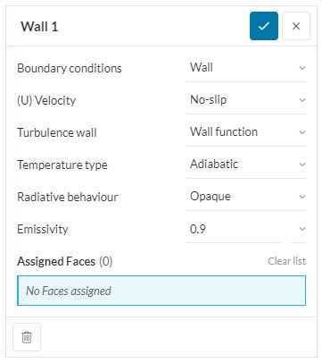
• Radiative behaviour: This input specifies the relationship between the net radiative heat per unit surface area, \(Q_r\), and the temperature of every surface, \(T_s\). In SimScale, you can set two radiative surface behaviors, transparent and opaque.
• Emissivity: Emissivity is a constant, which defines the ratio of thermal radiation from a surface to the radiation from an ideal black surface concerning the Stefan-Boltzmann law. The ratio varies from 0 to 1 (1 represents the ideal black body). The emissivity depends on many factors such as material, surface finish, surface temperature, wavelength, and angle. For simplicity, one can use commonly published emissivity values for common materials\(^1\):

Material type	Emissivity
Human skin	0.95
Wood	0.82 – 0.92
Soil	0.93 – 0.96
Vegetation	0.92 – 0.96
Black paint	0.98
White paint	0.9
Concrete	0.92 – 0.96
Copper, polished	0.04
Copper, oxidized	0.87
Brick	0.9

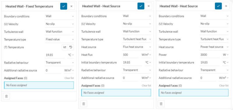
Heated Wall

A constant temperature, heat flux, or power source can be added to represent the behavior of heating or cooling walls. If the initial boundary temperature predicted by the user is closer to the final value, the solver will achieve convergence faster.

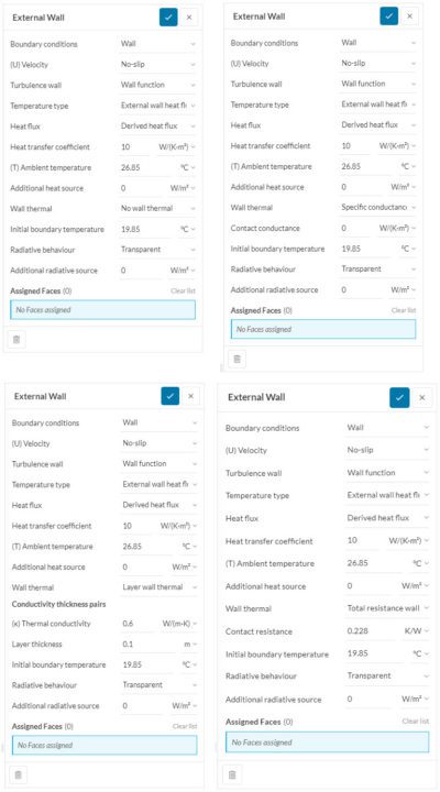
External Wall

External walls are walls assumed to be interacting often with ambient conditions. Often a considerable temperature difference exists, therefore a high heat transfer is expected.

• Heat transfer coefficient: Convection coefficient between the fluid surface and exterior surrounding;
• (T) Ambient temperature: Temperature of the exterior surrounding;
• Contact conductance: U-value of the wall. This is an overall heat transfer coefficient that measures the rate at which a building element transmits heat;
• (K) Thermal conductivity: Thermal conductivity of the wall material;
• Layer thickness: Thickness of the wall material.

There is a variety of options to determine the Wall thermal. This is an arbitrary wall between the fluid domain and the exterior that is added to work as thermal resistance. All the available ways to model this wall are listed below:

• No wall thermal: Wall is assumed to be too thin and/or conductivity is too high, so no wall resistance is expected.
• Specific conductance wall thermal: Building walls have multiple layers. Overall U-value of the wall is assigned to define a multilayered wall.
• Layer wall thermal: A single wall, with a single material. Thermal conductivity and layer thickness is assigned. Solver calculates resistance.
• Total resistance wall thermal: Thermal resistance is the ability of a material to resist the flow of heat, and the input here is the thermal contact resistance value of the wall. If you know the wall conductivity and thickness, or the U-value and external convection, along with the area of the surface, then you can calculate the contact resistance input.

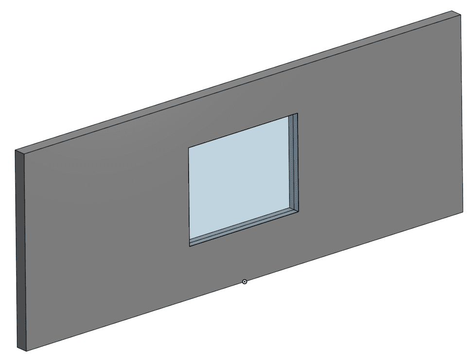
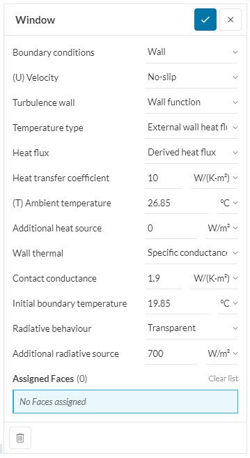
Windows

Windows can be defined similarly to walls, except the radiative behavior is different. SimScale does not differentiate the emissivity of different spectrums. Currently, we recommend assigning radiative behaviour as transparent. This will ensure that the window surface is not going to be included in radiative heat transfer.

With this kind of configuration, an Additional radiative source will release energy from the window surface via diffuse radiation, without changing the window temperature.

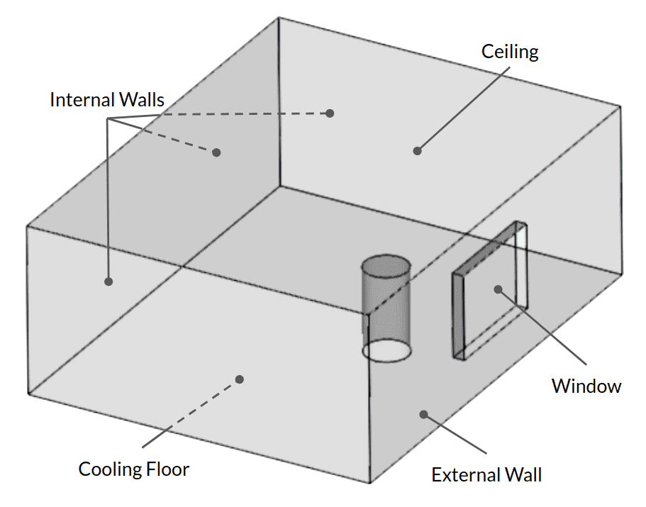
Expected Outcome

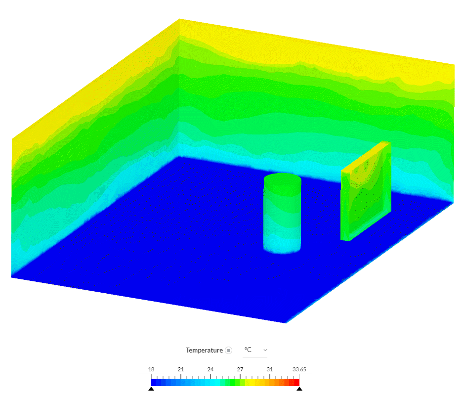
The following picture represents an example case to clarify the conditions explained above. Boundary conditions are defined as follows:

• Internal walls: Adiabatic wall, opaque
• Cylindrical obstacle: Adiabatic wall, opaque (this represents furniture, blocking the sunlight)
• External wall: External convection, a hot climate, a constant U-value, opaque
• Ceiling: External convection, a hot climate, a constant U-value, opaque
• Cooling floor: Constant temperature, opaque (this represents floor cooling system)
• Window: External convection, a hot climate, a constant U-value, transparent, additional radiative heat source

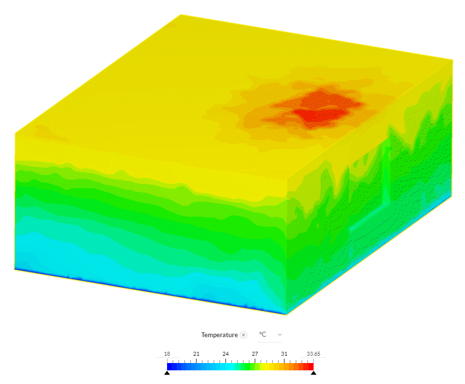
The temperature results clearly show the temperature gradient between the cold surface and the poorly insulated ceiling, which is exposed to hot ambient conditions. In front of the window, a high-temperature region is seen. This shows that there is a hot object below the ceiling in this region.

To be able to see the temperature on the walls more clearly, some walls and the ceiling are hidden. Now the floor, adiabatic walls, and the window are visible. One can notice that the frontal surfaces of the adiabatic obstacle look warmer than the other surfaces. The possible reason might be that the frontal surface receives radiation energy from the window.

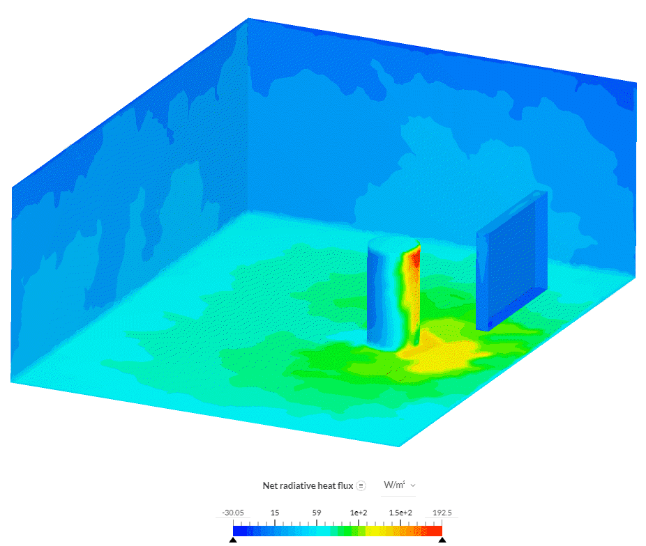
Net radiative heat flux contours show that the frontal surface of the cylinder receives most of the radiation energy. In addition, one can see that warmer objects (adiabatic wall and window) have a negative net radiative heat flux value, while colder objects (floor and cylinder) have a positive one. Finally, lower net radiative heat flux on the floor and behind the obstacle shows that furniture blocks the radiative energy dissipation coming through the window.

References

- Cengel, Y.A. (2002) Heat Transfer: A Practical Approach. 2nd Edition, McGraw-Hill, New York.