Advanced Tutorial: Thermal Comfort In a Meeting Room

This article provides a step-by-step tutorial for the full thermal comfort assessment in a meeting room using CFD simulation, including models for convective heat transfer, radiation heat transfer, and age of air.

PMV in a meeting room as result of thermal comfort simulation — Figure 1: Visualization of the thermal comfort parameter (PMV) in the meeting room

Overview

This tutorial teaches how to:

Set up and run a convective heat transfer flow simulation
Assign boundary conditions, material, and other models to the simulation
Mesh the geometry with the SimScale standard meshing algorithm
Set up scalar species transport analysis for the local mean age of air computation
Set up radiation heat transfer
Define thermal comfort parameters computation.

The typical SimScale workflow will be followed:

Prepare the CAD model for the simulation.
Set up the simulation.
Set up the mesh.
Run the simulation and analyze the results.

1. Prepare the CAD Model and Select the Analysis Type

First of all, click the button below. It will copy the tutorial project containing the geometry into your own Workbench.

Import Tutorial Into Workbench

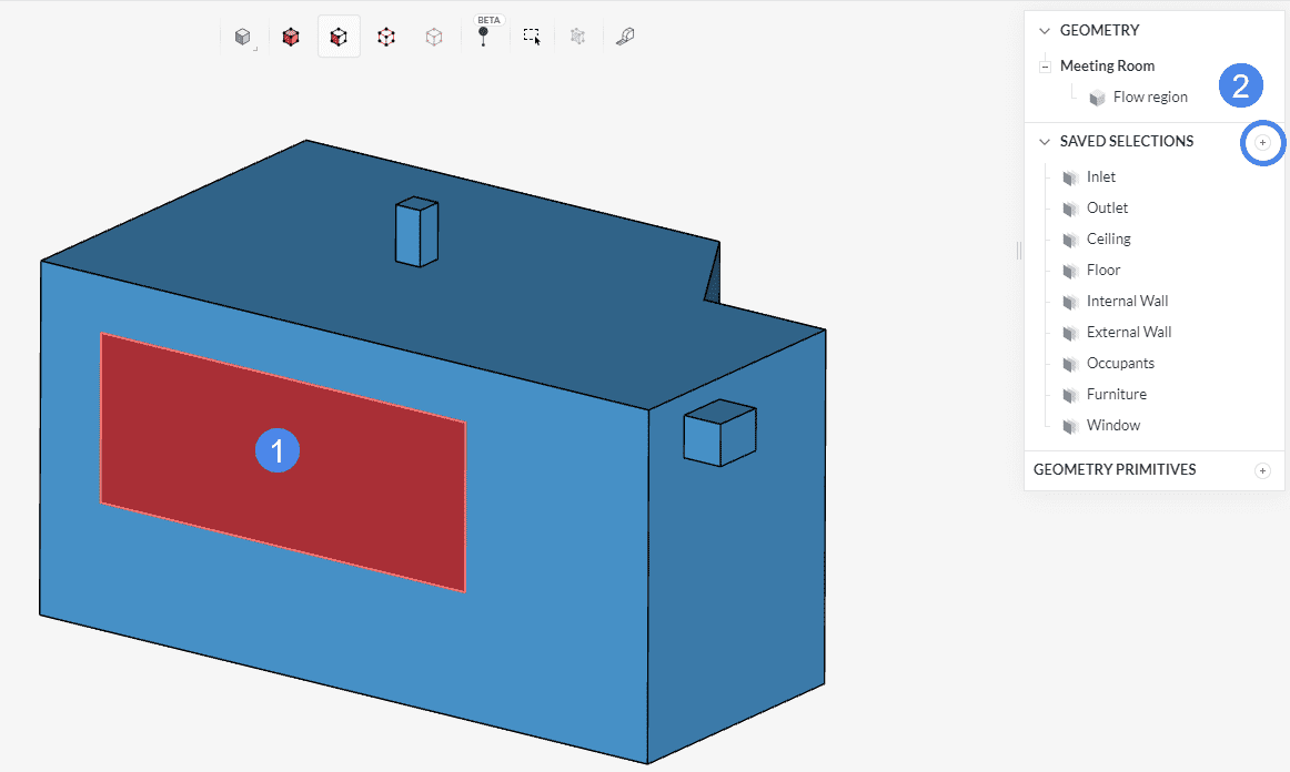
The following picture demonstrates what should be visible after importing the tutorial project.

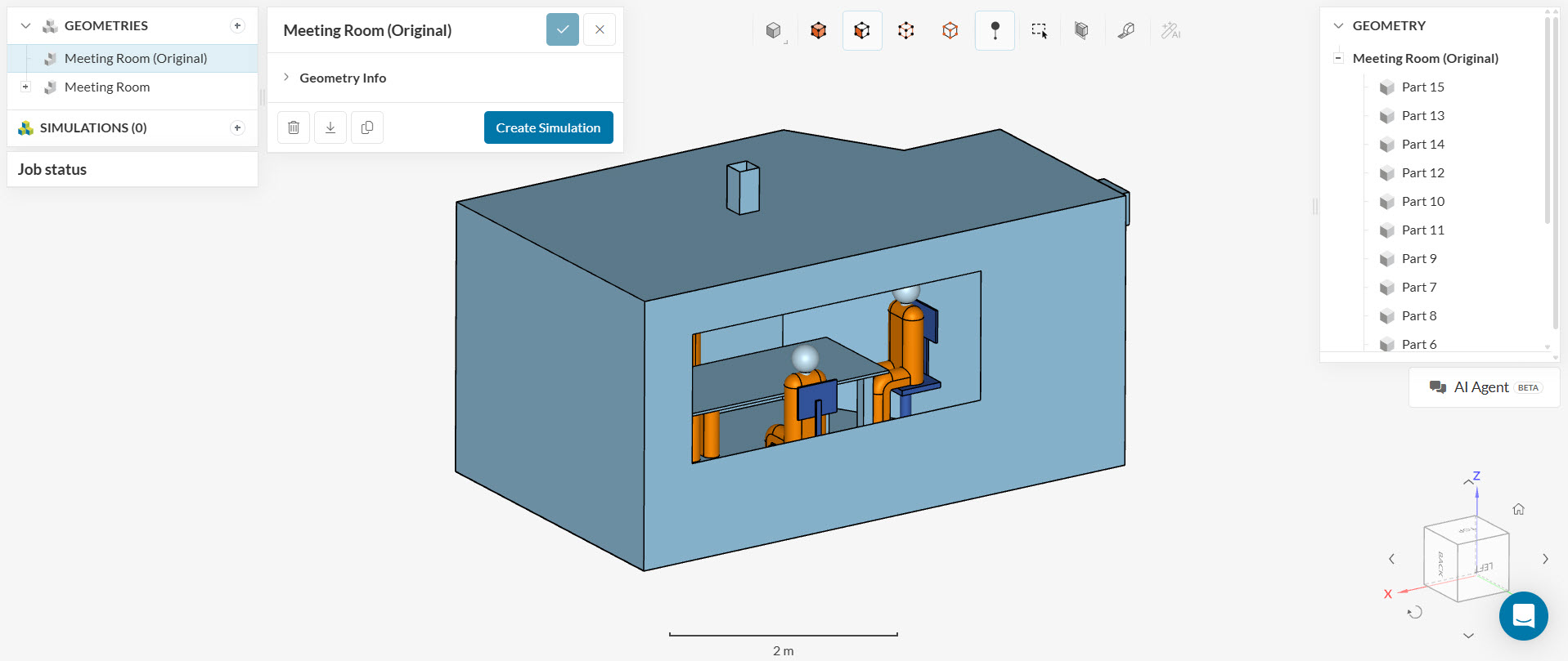
imported project in the simscale workbench for thermal comfort assessment — Figure 2: Imported CAD model of a meeting room in the SimScale Workbench

Please notice how the Meeting Room geometry consists only of a flow volume. As the original CAD model included the room walls, occupants, and furniture, an Internal flow volume operation was performed in CAD mode to create geometry for the volume of air. The volume of air represents the negative of the room and everything inside.

The original geometry without the flow volume extraction is included for comparison, under the name Meeting Room (Original).

Optional: Checking the flow volume extraction settings in CAD mode

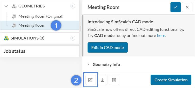
If you would like to see the internal flow volume operation settings in CAD mode, make sure to select the ‘Meeting Room’ geometry and press the ‘Edit in CAD mode’ button:

entering cad mode room tutorial flow volume creation — Figure 3: Entering the CAD mode environment to edit a geometry. The existing operations are listed in the left-hand side panel within CAD mode.

To exit CAD mode, simply click on the ‘Exit’ button on the top-right corner.

Important

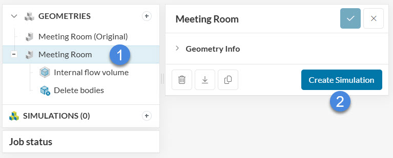
From now on, make sure you are working on the geometry with the flow volume extraction operation Meeting room, and not the original one presented for reference.

1.1 Create Saved Selections

Saved selections are groups of faces created at this point to be used in assignments for boundary conditions and other concepts, during the simulation setup. They can be found at the right-hand side panel:

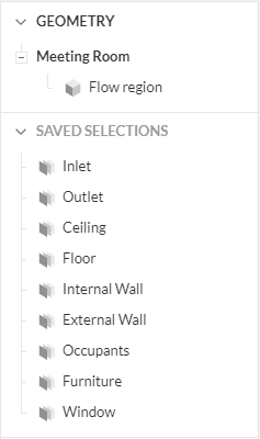
simscale topological entity sets for thermal comfort assessment — Figure 4: *Saved selections* appear on the right of the Workbench

A number of sets are already provided in the project, but one set for the window is still missing. The picture below shows how to add one:

creation of saved selections for thermal comfort assessment — Figure 5: Creating a saved selection for the window face

Create saved selections by selecting the Window face (highlighted in red),
Then click on the ‘+’ icon next to Saved Selections in the right panel.

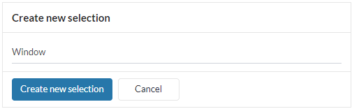
In the pop-up dialog that appears, name the set “Window” and click ‘Create new selection‘.

Note

Be sure that you have created all geometry operations before creating saved selections. If you do it the other way round, you will loose the sets.

1.2 Create the Simulation

Now we can start with the simulation setup. Follow the steps presented in the picture below to create a new simulation:

simulation creation for thermal comfort assessment — Figure 7: Creating a new simulation setup for thermal comfort assessment

Select the ‘Meeting Room’ geometry from the left panel,
then click the ‘Create Simulation’ button of the dialog:

The simulation library window appears:

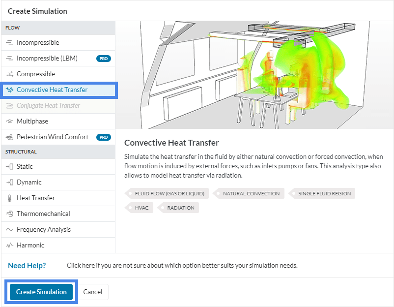
simulation type selection for thermal comfort assessment — Figure 8: SimScale simulation library

Here you can select the analysis type you need.

Choose ‘Convective Heat Transfer’ and click ‘Create Simulation‘.
Now, you will see a new simulation tree element with it’s default settings dialog open:

simulation setup — Figure 9: Global simulation parameters

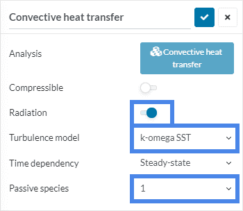
Perform the following changes:

Activate Radiation for the simulation.
Change turbulence model to ‘k-omega SST’.
Set Passive species to ‘1’ (This is necessary for the calculation of the age of air).

Do not forget to click the checkmark at the top to save the changes.

2. Set Up the Simulation

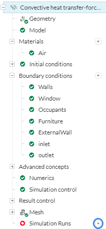
In order to have an overview, the following is a description of the simulation model and conditions:

model overview for thermal comfort assessment — Figure 10: Model overview

Heat transfer is performed through forced convection, natural convection, and radiation.
Conditions for summer with an ambient temperature of 30 \(°C\) and relative humidity of 65%
Output flow at the back duct, the inlet flow rate of 0.1 \(m^3/s\) and 18 \(°C\) at the top duct
The inlet flow rate of 0.1 \(m^3/s\) and 18 \(°C\) at the top duct
The radiation heat load of 200 \(W/m^2\) at the window
Conductive walls to an external temperature of 30 \(°C\) for the external walls and window
Adiabatic walls for the internal walls, ceiling, and floor
Flux power heat source of 40.79 \(W/m^2\) for the occupants metabolic rate
Adiabatic walls for the furniture
The age of air is modeled through the local mean age of air (LMA) model by the integration of a transported passive scalar.

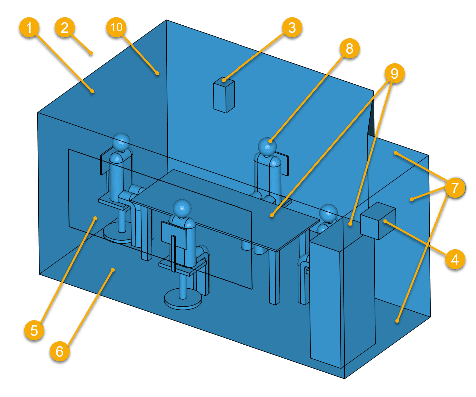
You can explore the corresponding faces for each condition by clicking the saved selections at the right panel.

Note

The above situation has some convection induced by the ventilation system and the window is considered to be closed. You will also find a version without forced ventilation by the ducts and the window considered to be open later in the tutorial.

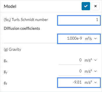
2.1 Global Model – Setting Up Age of Air

Select the Model tree element to specify the scalar transport properties and gravitational acceleration. For the LMA (local mean age of air) model, the following parameters are used:

model setup — Figure 11: Scalar transport and gravity model parameters

Turbulent Schmidt number: ‘1’.
Diffusion coefficient: ‘1e-9’.
And for Gravity, please set ‘9.81’ \(m/s^2\) in the negative Z direction.

2.2 Material

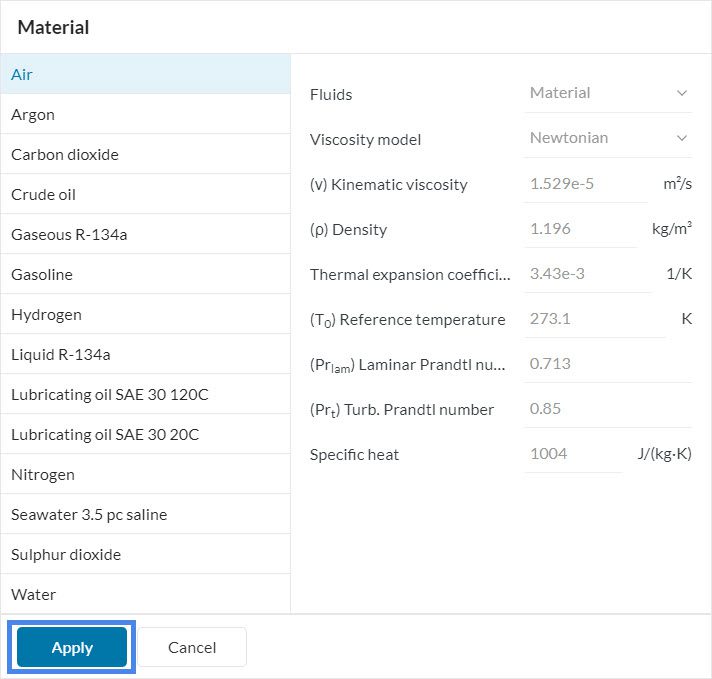
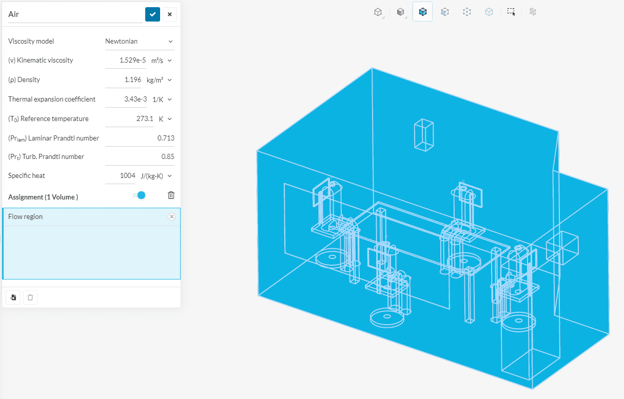
To define and assign a material, please click on ‘+’ next to Materials. Doing so, the SimScale material library will pop up:

simscale materials library for thermal comfort assessment — Figure 12: SimScale materials library

Select ‘Air’ from the materials library and click ‘Apply’.
As there is only one flow volume, it is automatically assigned.
Accept the selection with the check mark button.

choosing the material parameters for the air and flow region assignment — Figure 13: Material parameters for air and assignment of the flow region

2.3 Boundary Conditions

Now we need to set up the boundary conditions presented in Figure 10. Note that there are two versions of the setup:

Forced convection: The ventilation system provides airflow within the room and the window is considered to be closed.
Natural convection: The ventilation system does not provide airflow and the window is considered to be open.

However, we will start with the settings necessary for both scenarios, later on you can decide which scenario you want to simulate.

a. Internal Walls / Floor / Ceiling

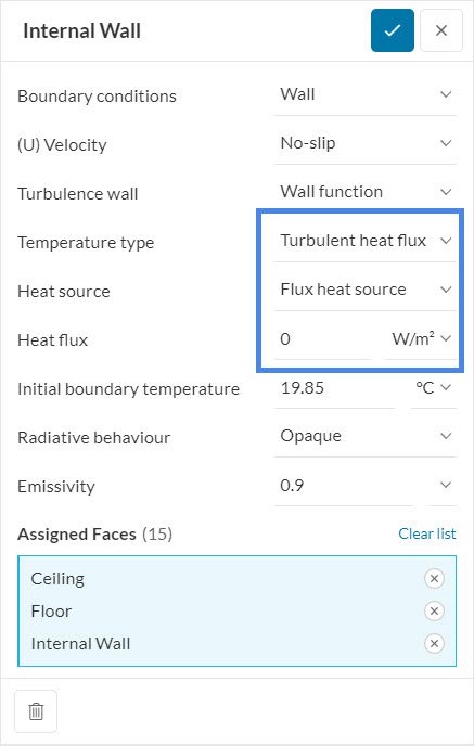
Internal walls are assigned as a wall boundary condition, and as they are facing the inside of the building, they are considered adiabatic.

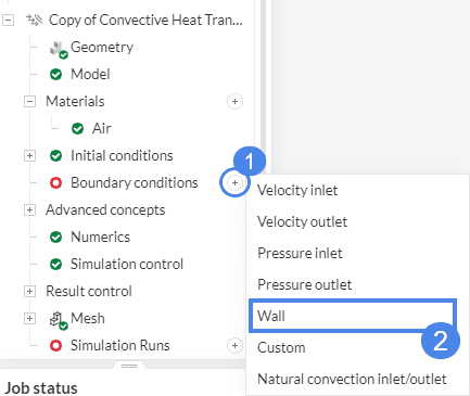
process explaining how to create a wall boundary condition — Figure 14: Create new boundary condition

Create a ‘Wall’ boundary condition and assign the Internal wall, Ceiling, and Floor sets, have a look at Figure 4 to see where to find the saved selections. Set up the parameters as shown in the reference picture:

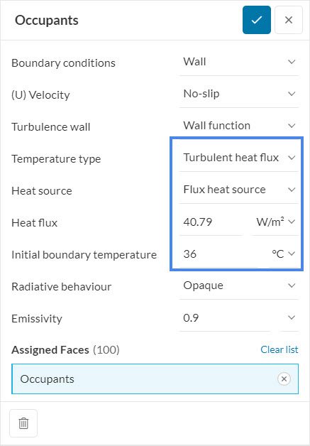
internal walls boundary condition for thermal comfort assessment — Figure 15: Assign the internal walls boundary condition

b. Occupants

For the occupants, a wall boundary condition is also used, this time with a heat flux power source to model the metabolic heat generation rate. Create a ‘Wall’ boundary condition and assign the Occupants set. Set up the parameters as shown in the picture:

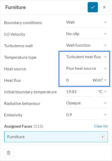
occupants boundary condition for thermal comfort analysis — Figure 16: Assign the occupants boundary condition

c. Furniture

For the furniture, a wall boundary condition is also used, with adiabatic thermal behavior. Create a ‘Wall’ boundary condition and assign the Furniture set. Set up the parameters as shown in the picture:

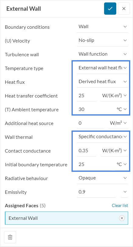
furniture boundary condition for thermal comfort assessment — Figure 17: Assign the furniture boundary condition

d. External Wall

For the external wall, a wall boundary condition is also used, with a thermal wall model and convection to the exterior. Create a ‘Wall’ boundary condition and assign the External Wall saved selection. Set up the parameters as shown in the picture:

external walls boundary condition for thermal comfort assessment — Figure 18: Assign the external wall boundary condition

The following articles provide additional information about thermal wall modelling:

You can add a natural convection setup to simulate a model without air conditioning, where the window is open for natural cooling, or a forced convection setup to simulate the scenario when the window is closed and the air conditioning is on.

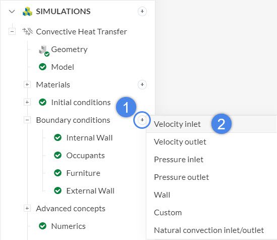
Version 1: Cooling with Forced Convection Boundary Conditions

a. Flow Inlet

A flow velocity inlet boundary condition is created according to the following picture:

boundary condition creation for thermal comfort assessment — Figure 19: Create new boundary condition

After hitting the ‘+’ button next to Boundary conditions, a drop-down menu will pop-up where different types of boundary conditions can be chosen.
Select ‘Velocity inlet’ from the list.

Now the setup for the velocity inlet boundary condition will pop up:

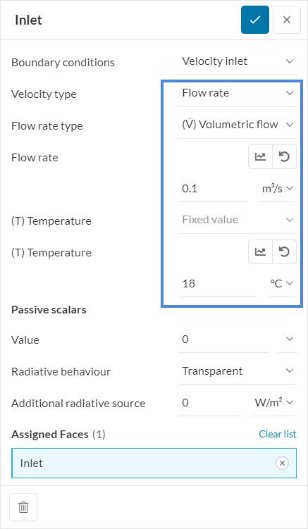
assigning the inlet velocity in simscale — Figure 20: Assigning the flow inlet boundary condition

Please modify the following:

Set a Volumetric flow rate of ‘0.1’ \(m^3/s\),
Temperature of ’18’ \(°C\),
Passive scalar remains at ‘0’ to model fresh air with zero LMA.
For the assignment, select the inlet face. You can find it as the predefined Inlet saved selections in the geometry tree on the right side of the Workbench.

b. Flow Outlet

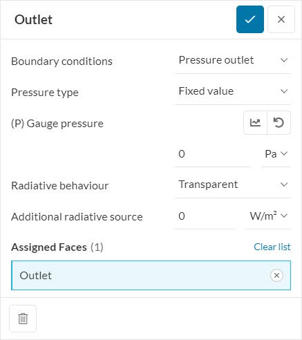
For the flow outlet boundary condition, follow the same procedure, but select a ‘Pressure outlet’. Leave all values as default and assign the Outlet set, as shown in the image:

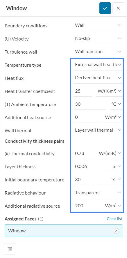
outlet boundary condition for thermal comfort assessment — Figure 21: Assign the pressure outlet boundary condition

c. Closed Window

For the window, a wall boundary condition is also used, but this time with a layer wall thermal model, convection to the exterior temperature, and an external radiation source to model sunlight. Create a ‘Wall’ boundary condition and assign the Window set. Set up the parameters as shown in the image:

window boundary condition for thermal comfort assessment — Figure 22: Assign the window boundary condition.

Version 2: Cooling with Natural Convection Boundary Conditions

a. Natural Convection Inlet/Outlet

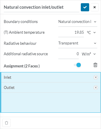
For the natural convection boundary condition, select ‘Natural convection inlet/outlet’. Assign the Ambient temperature as the expected temperature surrounding your model. Radiation effects on the inlet and outlet won’t be considered with the ‘Transparent’ radiative behavior applied.

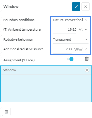
natural convection boundary condition for thermal comfort assessment — Figure 23: Assign the natural convection boundary condition.

b. Open Window

For the window, a natural convection boundary condition is used, similar to the one applied to the inlet and outlet faces but this time define the Additional radiative source as 200 \(W/m^2\) This setup takes into consideration an external radiation source to model sunlight and the open boundary conditions allowing the air to circulate through the surface in both directions:

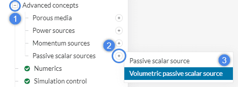
open window boundary condition for thermal comfort assessment with additional radiative source — Figure 24: Assign the open window boundary conditions

2.4 Advanced Concepts

Under advanced concepts, you can define further advanced physical conditions to set up your simulation. For this tutorial, you need to define a passive scalar source.

a. Passive Scalar Source

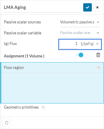
For the LMA aging model, a ‘Volumetric passive scalar source’ is used, as shown in the image:

volumetric passive scalar source for thermal comfort assessment — Figure 25: Volumetric passive scalar source concept

Expand Advanced concepts,
Click the ‘+’ button next to Passive scalar sources,
Select ‘Volumetric passive scalar source’.

Assign the flow region to the concept and specify a Flux value of 1.

local mean age of air aging setup for thermal comfort assessment — Figure 26: Volumetric passive scalar source parameters

For thermal comfort simulations, these options might be interesting:

Power sources: With those, you can define additional power sources to volumes. If you do not have the corresponding volume in SimScale use geometry primitives.
Momentum source: You can utilize those to model fans. They are also applied to a volume. They accelerate the flow to a specified velocity and direction.

2.5 Numerics and Simulation Control

For the numeric solver parameters, the only change made is the addition of non-orthogonality correctors. This will improve the convergence for the tetrahedral mesh created by the Standard mesher algorithm. Setup the Number of non-orthogonal correctors as shown in the picture:

numeric setup for thermal comfort assessment — Figure 27: Numerical parameters

Click on ‘Numerics’ to display the solver parameters.
Set the Number of non-orthogonal correctors to ‘4’.

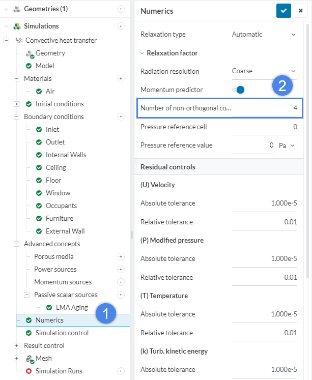
Setting Relaxation type to ‘Automatic’ might speed up the convergence. Consider this option if there are divergence issues.

Regarding Simulation control, we keep the setup to the default values.

2.6 Result Control Items

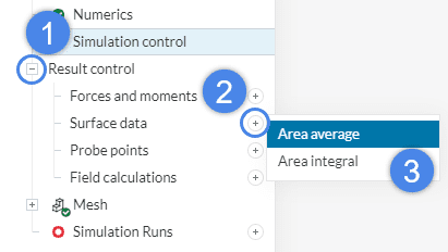
Result control items are used to retrieve specific computations from the numerical solver. By using them, we can have a look at specific variables at specific regions by querying the computation and output of our quantities of interest.

a. Local Mean Age of Air

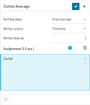
In order to measure the average LMA at the outlet face, a Result control item is used. It is created as shown in the picture:

area average result control creation for thermal comfort assessment — Figure 28: Area average result control item creation

Expand Result control,
Click the ‘+’ icon next to Surface data,
Select ‘Area average’.

Assign the Outlet set and check that the setup coincides with the picture:

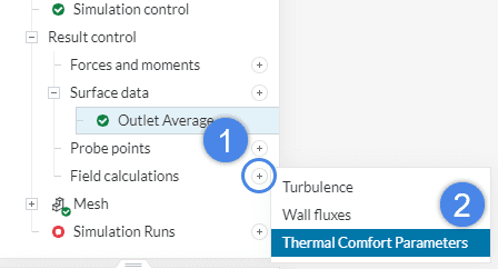
area average result control setup for thermal comfort assessment — Figure 29: Area average result control item parameters

b. Thermal Comfort Parameters

Thermal comfort parameters are also queried in the result control items, under Field calculations. Create the concept as shown in the picture:

thermal comfort parameters creation for thermal comfort assessment — Figure 30: Thermal comfort parameters creation

Click the ‘+’ button next to Field calculations,
Select ‘Thermal Comfort Parameters’.

Set up the parameters as shown in the picture:

thermal comfort parameters setup for thermal comfort assessment — Figure 31: Thermal comfort parameters setup

In this case, the Clothing coefficient is ‘0.5’,
the Metabolic rate is ‘1.0’,
and the Relative air humidity is ‘65%’.

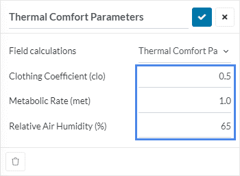
A description of the computed quantities and resulting fields can be found on this SimScale documentation page: Thermal Comfort Parameters.

3. Mesh

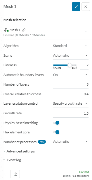
In the mesh setup, change Fineness to ‘7’. Under Advanced settings set the Small feature suppression to ‘0.004’ \(m\). You do not need to click Generate, as the mesh will be computed as part of the simulation run.

mesh parameters setup — Figure 32: Mesh parameters

4. Start the Simulation

Now that the simulation setup is complete, a new ‘Simulation Run’ can be created to perform the computation. In the following picture, the whole tree setup is shown, and the item to create the simulation run is highlighted:

simulation run creation — Figure 33: Simulation setup tree for forced convection before starting the simulation

In the pop-up window, press ‘Start’ to immediately begin the computation run. If the software predicts a higher duration of simulation and exceeding maximum runtime you can choose to ignore it or go back to simulation control settings and increase the maximum runtime value.

The computation takes around one and a half hours to complete. If you can’t wait to see the results, at the end of the article there is a link to the completed version of the project.

5. Post-Processing

We will use the integrated post-processor to visualize the temperature inside the meeting room, evaluate the thermal comfort of the room by visualizing the Percentage Mean Vote (PMV), and the local mean age of the air.

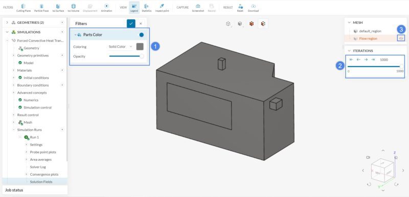
Before starting to post-process the results, make sure that there are no predefined filters. You can delete existing filters at any time by clicking on the dustbin icon next to them. Furthermore, please ensure that you are at the last timestep of your simulation by sliding the Iterations selector all the way to the right. Lastly, hide the Flow region in the MESH dialog by clicking on the ‘eye’ icon.

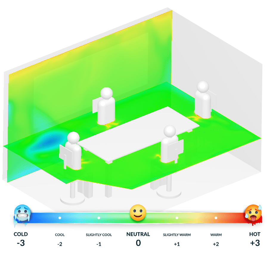
post-processor user interface — Figure 34: Make sure that there are no predefined filters, you are at the last timestep of the simulation and hide the **‘Flow region’** in the *MESH* dialog.

5.1 Temperature

Visualize the temperature by selecting ‘Temperature’ as the Coloring for your parts. Change the units of temperature to Celsius by clicking the units in the legend and selecting ‘°C’ and change the maximum temperature visualized to ’40’ \(°C\). Hide the walls of the room by selecting them and right-clicking on your mouse to select ‘Hide selection’. The temperature distribution inside the room can be seen in the figure below:

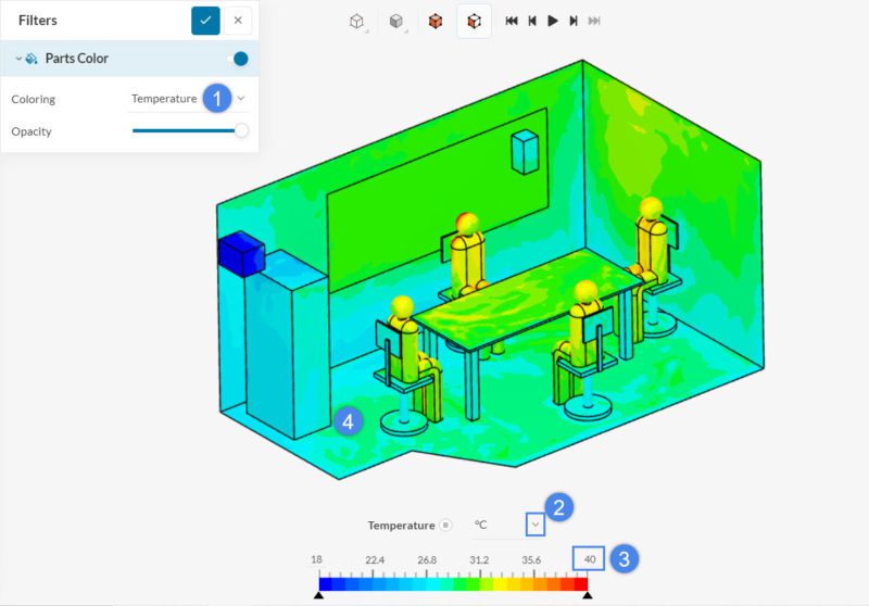
temperature distribution in a meeting room — Figure 35: Temperature distribution on the surfaces of the meeting room and the people sitting inside

From the figure above, we can see that the bodies emit heat and that the temperature increases as it is further from the inlet. The room is unevenly heated with the floor being slightly cool to neutral as we progress towards the ceiling where it is slightly warm.

5.2 Predicted Mean Vote (PMV)

Next, we will focus on visualizing the thermal comfort parameters, which are the predicted mean vote (PMV) and predicted percentage dissatisfied (PPD). The thermal comfort parameters will be visualized by using the cutting plane filter. Follow the steps below to create a cutting plane:

cutting plane settings for hvac in meeting room — Figure 36: Cutting plane settings at mid-height of the meeting room showing **‘Predicted Mean Vote (PMV)’**

Select the filter of interest from the top ribbon to create a new filter
Configure the cutting plane, so that it is placed at the mid-height of the room. Adjust the Position of the cutting plane by using the following coordinates: ‘2.35, 0.5, 0.785’. The Orientation of the cutting plane should be in the ‘Z’ axis and change the Coloring to the ‘Predicted Mean Vote’. Disable the Clip model slider, so that the model is not clipped.

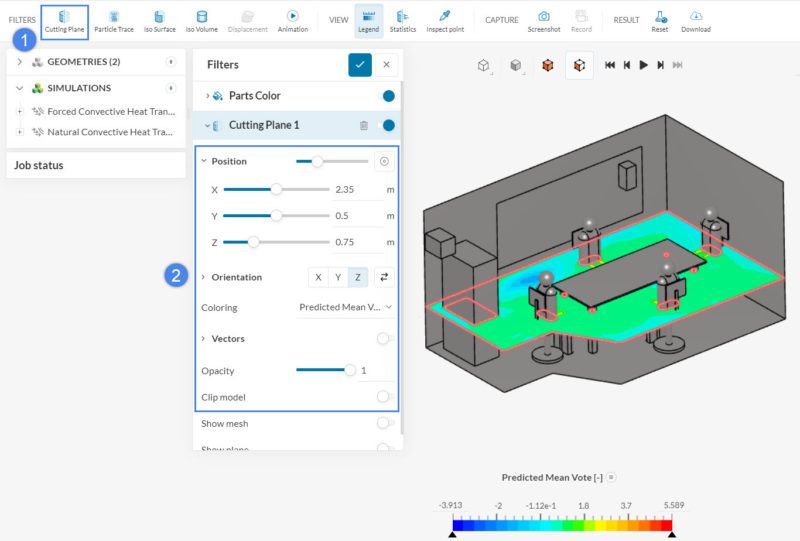
Using the same approach from above, create a second cutting plane normal to the ‘X’ axis. The predicted mean vote (PMV) thermal comfort index distribution is displayed in the following picture:

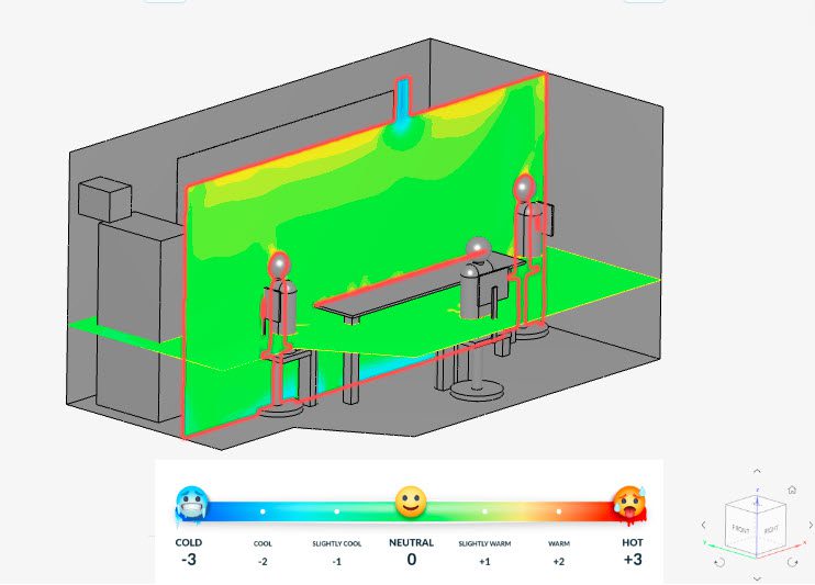
predicted mean vote in the room — Figure 37: Predicted mean vote (PMV) index distribution in the room

The value of the index is clipped to the recommended range of [-3, 3]. This way, we can visualize the areas that are below and above them, with blue and red colored regions respectively.

5.3 Local Mean Age (LMA) of Air

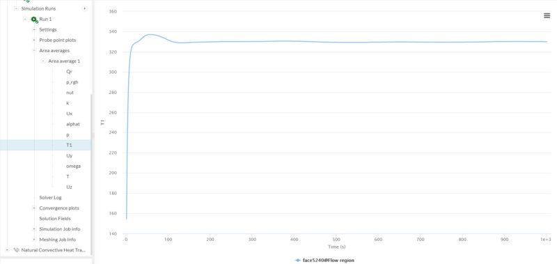
You can access the Local Mean Age (LMA) by selection ‘T1’ under Area average 1 in the simulation run, which calculates the average quantities at the outlet. The Local Mean Age (LMA) was computed at around 330 seconds for the forced convection scenario:

local mean age of air lma on outlet face for thermal comfort assessment — Figure 38: Mean age of air convergence at outlet face was computed to be around 330 seconds

The distribution of the LMA across the room can also be visualized using cutting planes. Add the velocity vectors by sliding the slider besides Vectors and change the Coloring to black Solid color, with a Scale factor to ‘0.5’.

The settings for the cutting plane in the y-axis and the final distribution for the LMA can be observed as below:

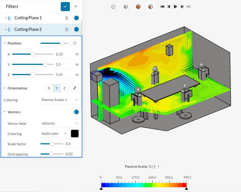
local mean age of air on perpendicular planes in simscale post processor — Figure 39: Mean age of air on two perpendicular cutting planes with velocity vectors to show airflow inside the meeting room. Blue regions depict fresh air while red ones depict air with poor ventilation.

Blue regions show areas with fresh of air and red regions show areas with high age of air. Red areas represent stagnation regions, with poor ventilation.

Analyze and explore your results with the SimScale post-processor. Have a look at our post-processing guide to learn how to use the post-processor.

Congratulations! You finished the tutorial!

Have a Look at the Finished Project

Last updated: September 27th, 2023

Did this article solve your issue?

How can we do better?

We appreciate and value your feedback.