Advanced Tutorial: Wind Analysis Simulation using the LBM (Lattice Boltzmann Method) Solver
This article provides a step-by-step tutorial on how to configure a wind analysis simulation with SimScale by using the LBM solver.
Note
This tutorial uses the Lattice Boltzmann Method (LBM), provided by Numeric Systems GmbH (Pacefish®)\(^1\), to solve the simulation. Since this solver is only accessible through professional licenses, this tutorial cannot be performed using a community license – Learn more.
If you want to perform external aerodynamics with a community license, please check out the external aerodynamics section of the
main tutorial page.
Overview
This tutorial will teach you how to:
- Configure and run a simulation using the LBM solver.
- Create relevant geometry primitives in SimScale.
- Assign boundary conditions, material, and other relevant properties for the simulation.
- Mesh with the automatic mesher.
- Use the post-processor and obtain results of interest.
We are following the typical SimScale workflow:
- Prepare the CAD model for the simulation.
- Set up the simulation.
- Set up the mesh.
- Run the simulation and analyze the results.
1. CAD Preparation and Analysis Type Selection
First of all, click the button below. It will copy the tutorial project containing the geometry into your Workbench.
The tutorial project contains a CAD model from the Gangnam District, in Seoul. Here is a view of the Workbench after importing the project:
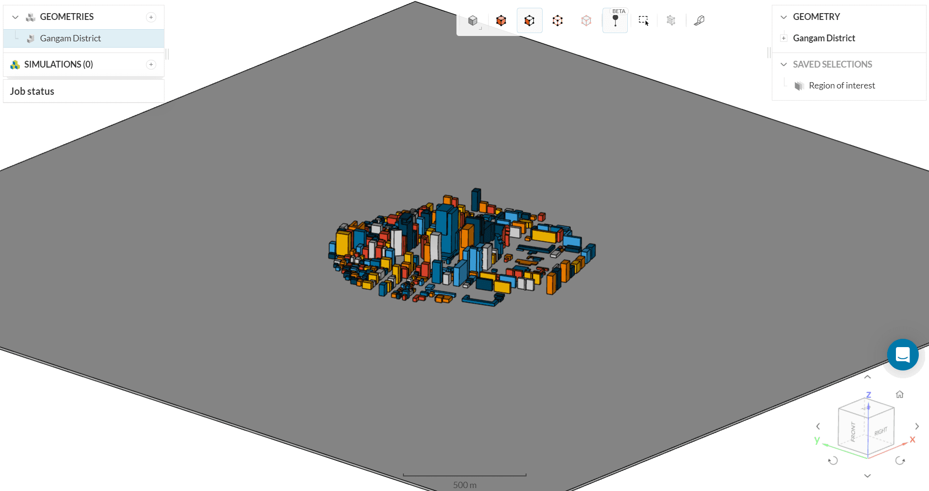
Importing new geometries to SimScale is just as easy. You can upload the geometry from your local machine or import it from Onshape® directly. Please visit the CAD preparation & upload page for further details.
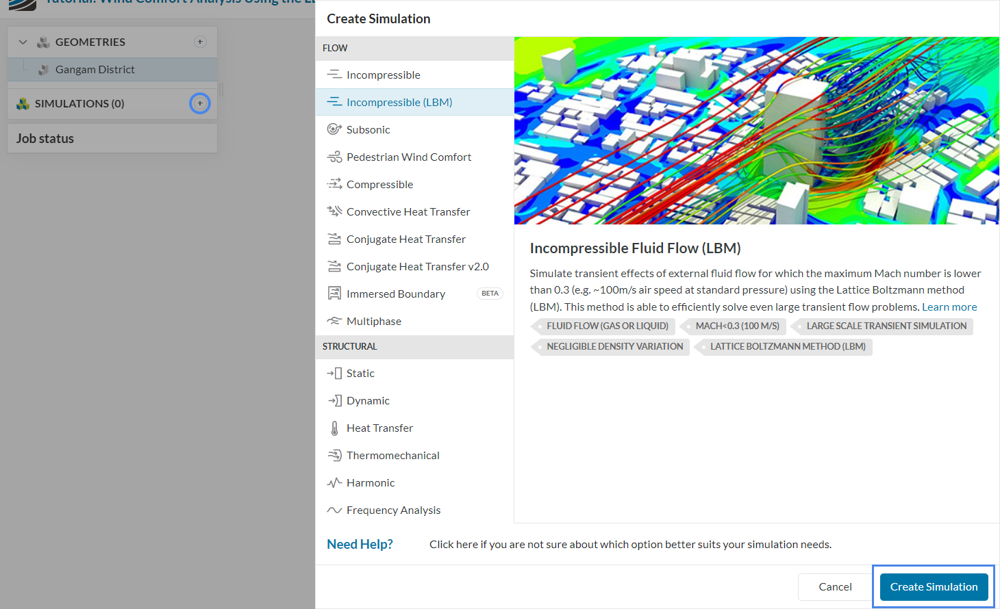
To create a simulation, click on the ‘+’ button next to Simulations and select ‘Incompressible LBM’ from the list. By clicking on ‘Create Simulation’, a new simulation tree appears in the left-hand side panel.
Did you know?
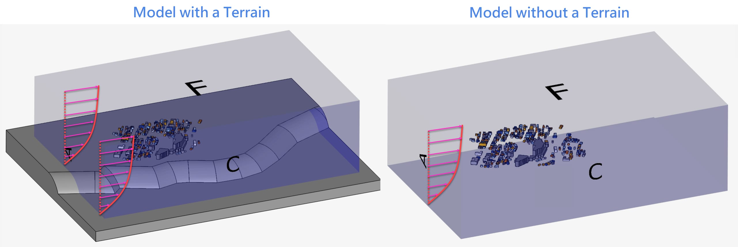
The LBM solver can deal with many CAD types and is more robust than many solvers in meshing the geometry. Open geometry with poor and small faces does not affect the meshing operation. However, if you do encounter issues or errors, an STL can normally be uploaded which may mitigate any issues that you experience.
2. Simulation Setup
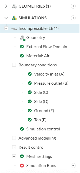
Users can set up their simulations in SimScale directly in the simulation tree. In the following sections, we will go through the necessary steps.
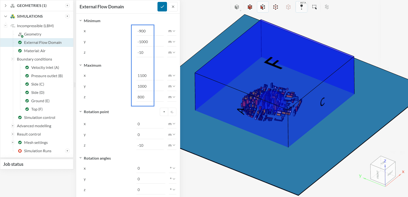
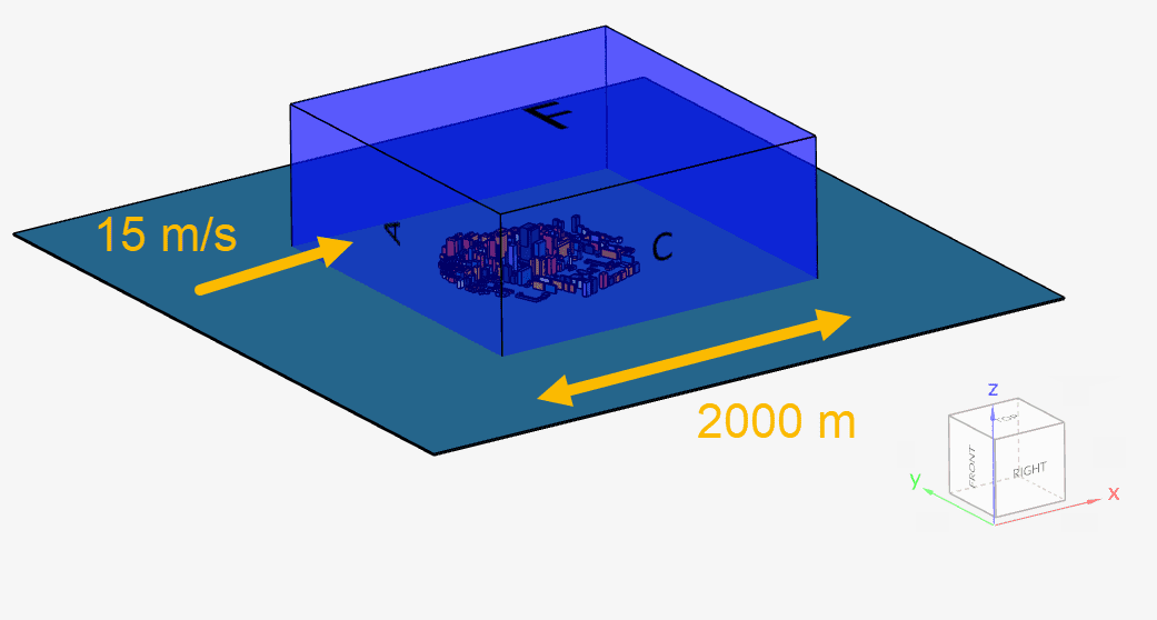
2.1. External Flow Domain
The first setting to address is the External Flow Domain dimensions. The external flow domain represents the computational domain, where the LBM solver calculates the solution. For this reason, it’s important to adequately size the flow domain, allowing a more accurate solution. This documentation page is a good reference for the flow domain size.
Did you know?
Evaluating flow from different directions is very easy in SimScale. It is possible to rotate the flow domain by using the rotation angles option. Please note that the right-hand rule applies -see the orientation cube in the bottom-right of the viewer for reference.
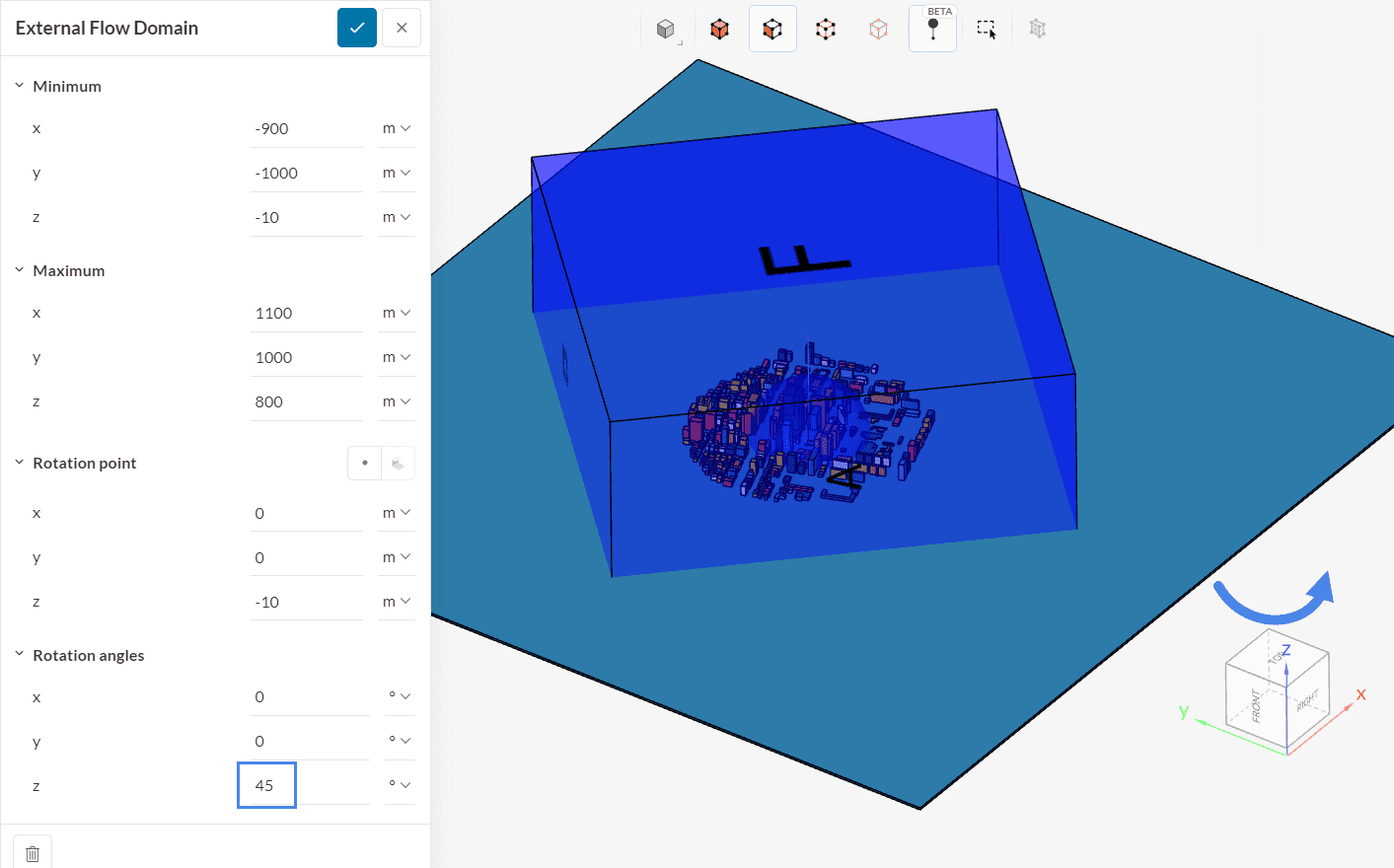
In this tutorial, we will maintain a rotation of zero degrees.
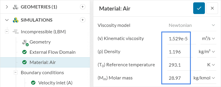
2.2 Material
Since this is a wind analysis simulation, the platform automatically assigns air to the domain. This tutorial uses the default air settings, however, it is possible to adjust the properties of air, such as density. To do so, simply select the field and edit the respective values:
2.3 Boundary Conditions
To run a simulation, it’s necessary to define the fluid conditions at the boundaries of the flow domain. Intending to streamline the simulation setup, the platform automatically assigns a default set of boundary conditions when you create a new simulation tree. The assumptions are:
- The sky is in the positive z-direction
- For an unrotated flow domain, the air flows from the negative to the positive x-direction
Using a CAD model with the orientations explained above will allow you to use the default boundary conditions with minimal adjustments. The image below shows an overview of the boundary conditions for this tutorial.
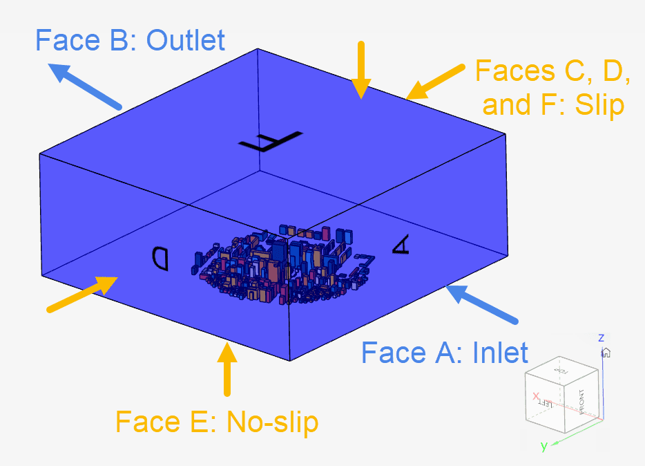
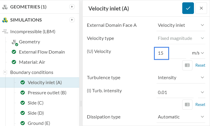
In this tutorial, we will only adjust the velocity inlet boundary condition.
For the velocity inlet configuration, please adjust the (U) Velocity to ’15’ \(m/s\):
To allow the definition of Atmospheric Boundary Layers (ABL), the velocity inlet boundary condition accepts table inputs (via .csv files) for the following parameters:
- Velocity as a function of height
- Turbulent Kinetic Energy or Intensity as a function of height
For interested readers, the following article discusses the ABL definition in greater detail:
Important
When defining an ABL profile via a .csv file, make sure that 0 meters represent the ground height.
2.4 Simulation Control
In the Simulation control settings, the user defines two parameters:
- End time: This parameter represents how many seconds of fluid flow the simulation will calculate
- Maximum runtime: This is the maximum simulation runtime in real-time. For example, if you set this value to 3600 seconds, the simulation will automatically stop after 1 hour of real-time has passed.
For this reason, it’s a good practice to set a large enough Maximum runtime to prevent the simulation from canceling. As for the End time, the recommendation is to allow at the very minimum 2 fluid passes (and optimally at least 3) through the domain. The figure below shows how you can calculate the End time of your simulation:
The formula to calculate the amount of time necessary for two fluid passes is simple:
$$End\ time = 2\ \frac{Domain\ size\ in\ flow\ direction}{Velocity} = 266.67\ seconds \tag{1}$$
2.5 Result Control
The Result control definition is critical for an Incompressible LBM simulation. Here, the user specifies what kind of information they want to receive in the results. For a complete description of all result control settings, please visit the following page.
In this tutorial, we will monitor forces and moments on faces of interest, and will also define a number of probe points that read the velocities at the pedestrian level.
a. FORCES AND MOMENTS
To monitor forces and moments about faces of interest, you can create a new Forces and moments result control. We will track the forces applied to two faces of the tallest building in the domain:
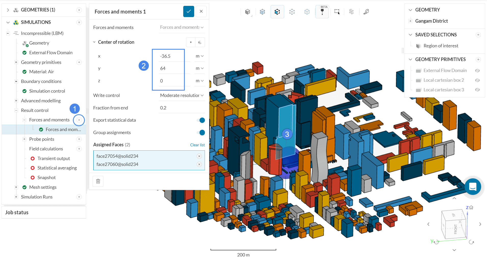
- Under Result control, click on the ‘+’ button next to Forces and moments
- Adjust the Center of rotation coordinates to the base of the building
- Lastly, select the faces of interest by clicking on them
b. PROBE POINTS
Probe points are also very useful for wind-related studies. With them, you can conveniently track the results at points of interest within the domain. In this tutorial, we will track the 10 points defined in the .csv file linked below:
Note that the .csv file consists of 4 columns, the first one containing the probe point name, and the remaining columns being the x, y, and z-coordinates of the point. After downloading the file, please follow the steps below:
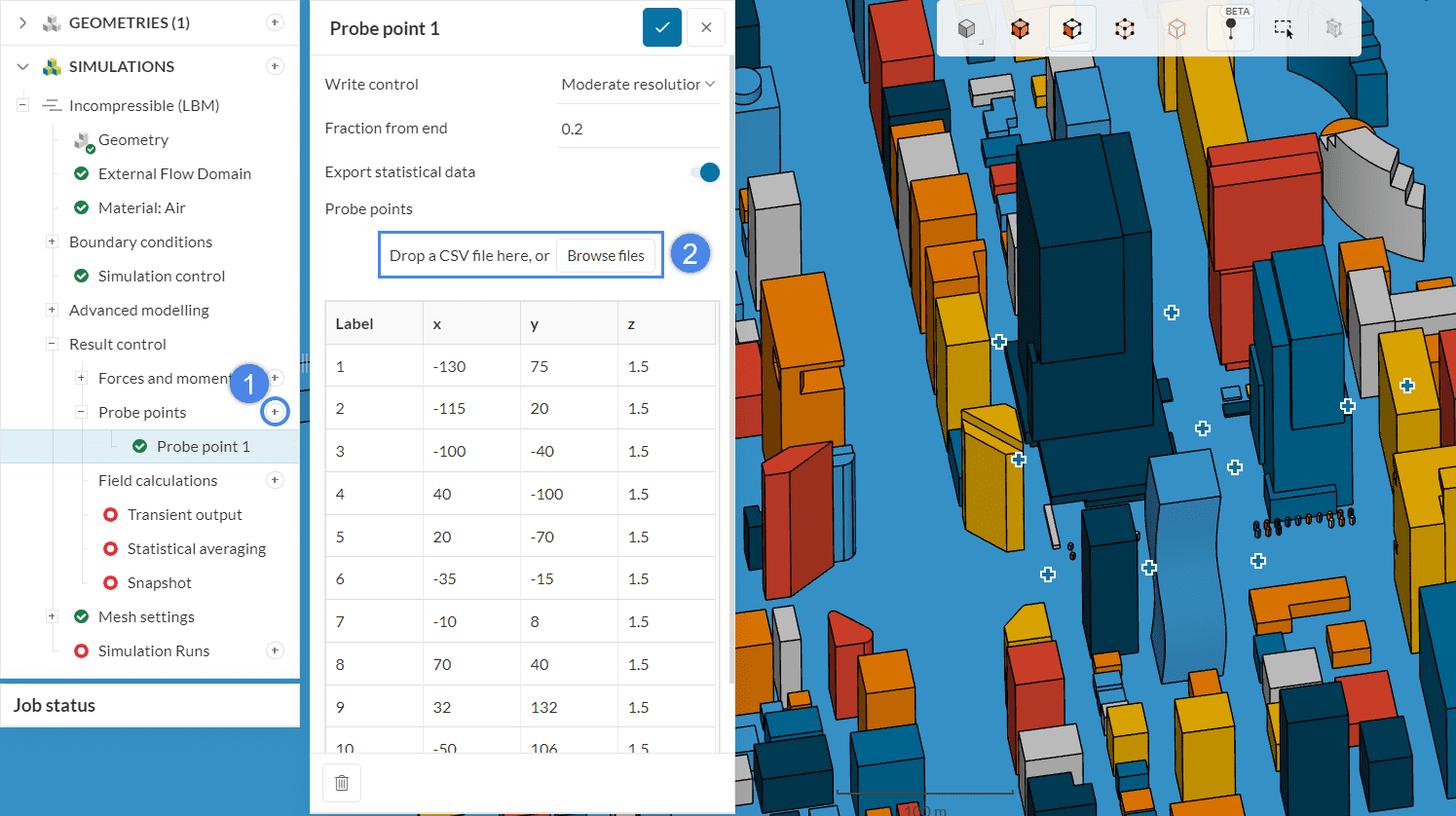
- Click on the ‘+’ button next to Probe points
- Drop the .csv file in the box
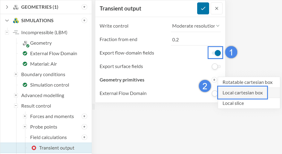
c. TRANSIENT OUTPUT
Under Transient output, you can define:
- The information to export (Surface fields and/or Flow-domain fields)
- Which regions will have their results exported
- Frequency of the data export
First, we will define the region to export. Therefore, click on the ‘+’ button next to Geometry primitives and choose a ‘Local cartesian box’ from the list:
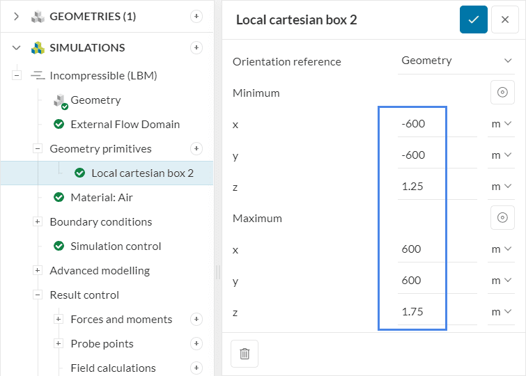
Now, you can define the coordinates of interest for the box. Defining a large box can cause problems with memory since transient simulations generate a lot of data. For this reason, we will focus on the pedestrian level:
After saving the settings, make sure to assign the local cartesian box to the transient output:
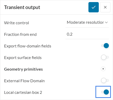
With these settings, the solver will export every 4th timestep result (Moderate resolution), during the final 20% of the simulation (Fraction from end).
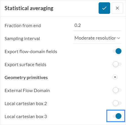
d. STATISTICAL AVERAGING
With Statistical averaging, the solver obtains mean values for all fields. To do that, it averages out the transient results from the final Fraction from end. Furthermore, the Sampling interval controls the frequency of the sampling.
Additionally, you can choose to export the results on the flow domain and/or on the surfaces. Following the steps from Figure 14, create another ‘Local cartesian box’, this time with the coordinates shown below:
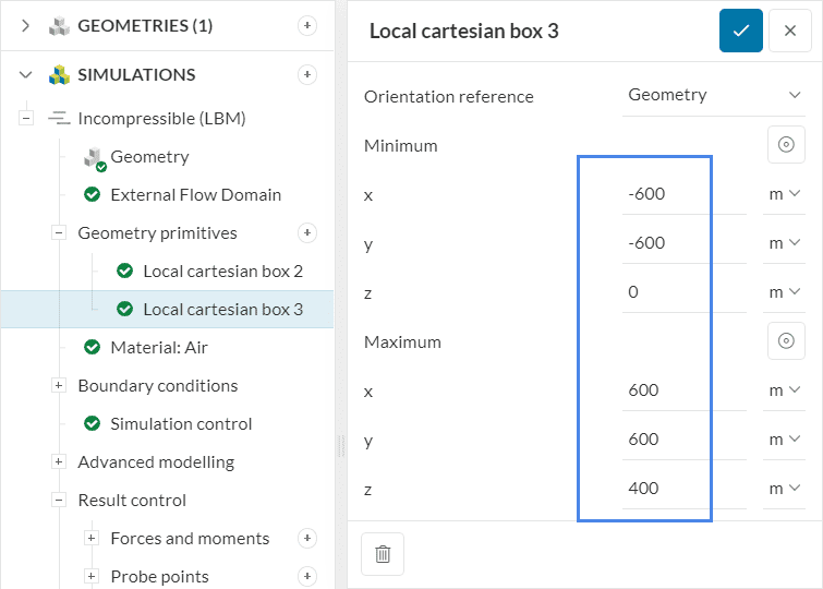
After saving the geometry primitive, make sure to assign it to Statistical averaging:
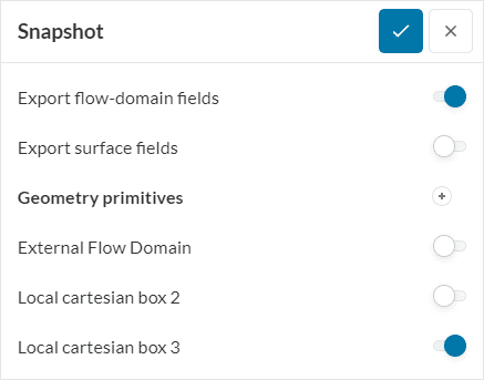
e. Snapshot
Snapshots take the last timestep of the simulation and export the instantaneous result fields for the fluid volume and/or surface data. Please assign the previous local cartesian box to it.
3. Meshing
The meshing tool for LBM simulation is powerful and easy to set up. In this tutorial, we will use the Automatic settings. In this setup method, the user defines the global level of Fineness and the Region of interest. It’s also possible to set additional refinements if required.
The Region of interest in this tutorial is the tallest building located in the center of the domain. To simplify the setup, this demonstration project contains a Saved Selections set with the faces of interest. Therefore, please expand the Saved Selections tab on the right-hand side panel, and assign the ‘Region of interest’ set:
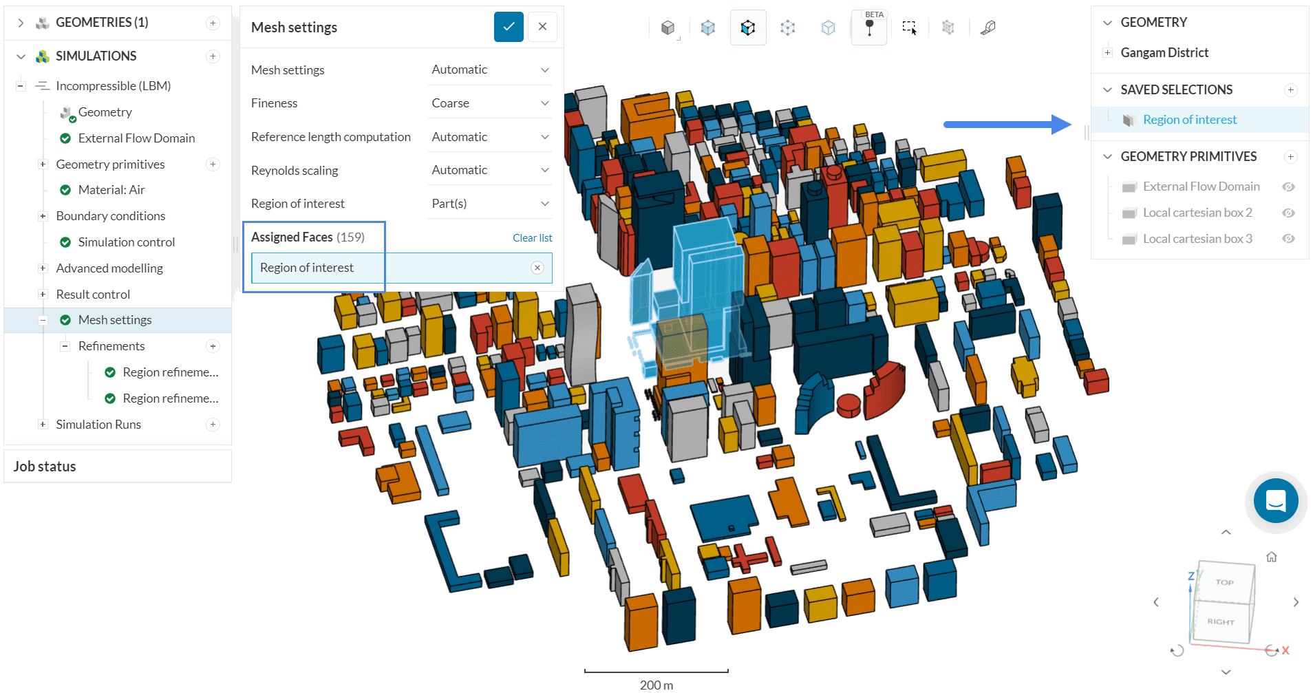
Furthermore, the pedestrian level is also of interest. To ensure a finer mesh, let’s create a region refinement as in the image below:
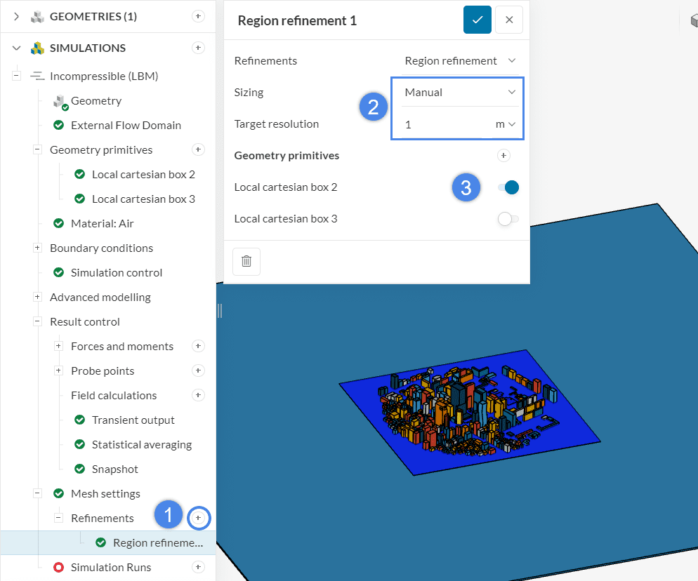
By defining a manual Target resolution, you ensure that the edge length of the cells within the cartesian box is not larger than ‘1’ meter. Now, create a second region refinement with a manual target resolution of ‘8’ meters, assigning it to Local cartesian box 3.
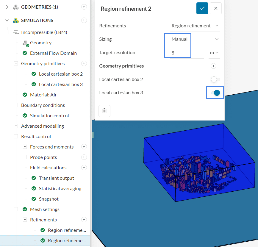
Region refinement settings for an LBM simulation are described more in detail on this page: Region Refinement Settings.
4. Simulation and Results
4.1 Run the Simulation
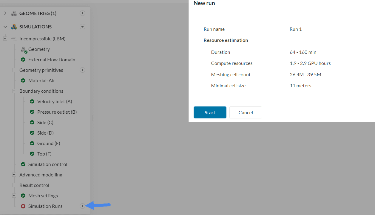
After finalizing the simulation setup, you can start a simulation run by pressing the ‘+’ button next to Simulation Runs.
4.2 Post-Processing
After the simulation finishes running, please expand the simulation run tab -you can access all the post-processing results from the simulation tree:
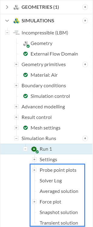
As a reminder, the results available to you depend on the Result control settings.
a. TRANSIENT SOLUTION
You will have the full capability of SimScale’s Post-Processor to analyze your simulation results, however, we will focus on the transient solution in this tutorial.
With the transient results, you can get time-dependent information and create animations. This allows you to visualize how the flow behaves within the regions of interest. As soon as the transient results load, you will see the following default configuration:
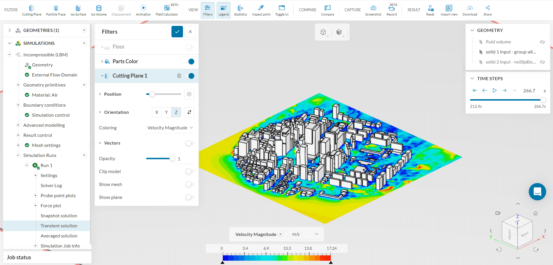
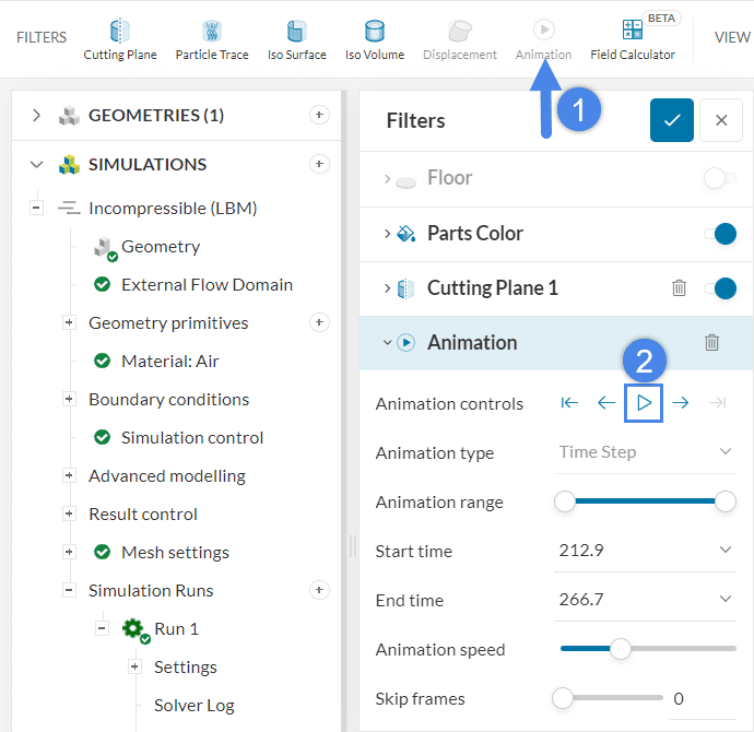
By default, the transient solution shows the results for a given time step. You can use the right-hand side TIME STEPS tab to navigate through the data sets. Another option is to create an ‘Animation’ filter to generate a smooth animation with the time-dependent solution:
Find below a video showing the animation results:
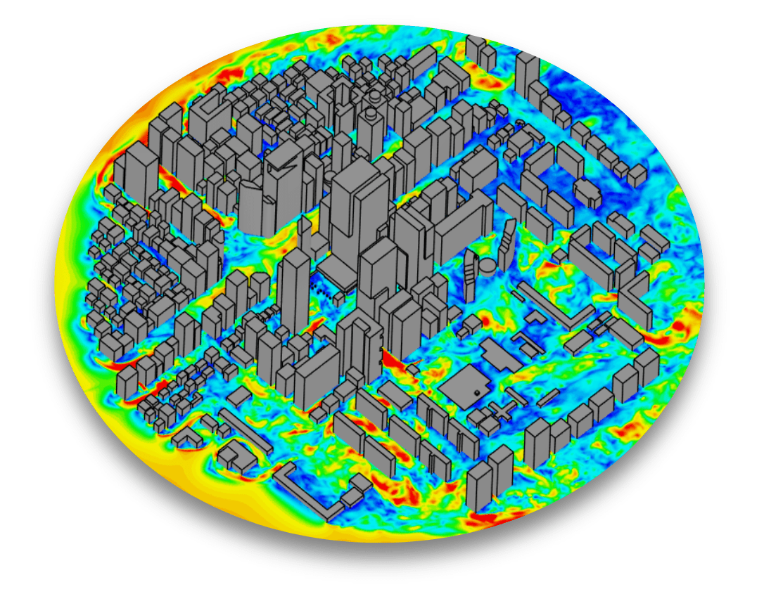
With the animation results, you can spot regions with high velocities, which can cause discomfort to pedestrians.
b. PROBE POINTS
The results are visualized in a temporal plot and a statistical summary. Additionally, you can also download the probe point data by clicking on the top-right icon from the image below:
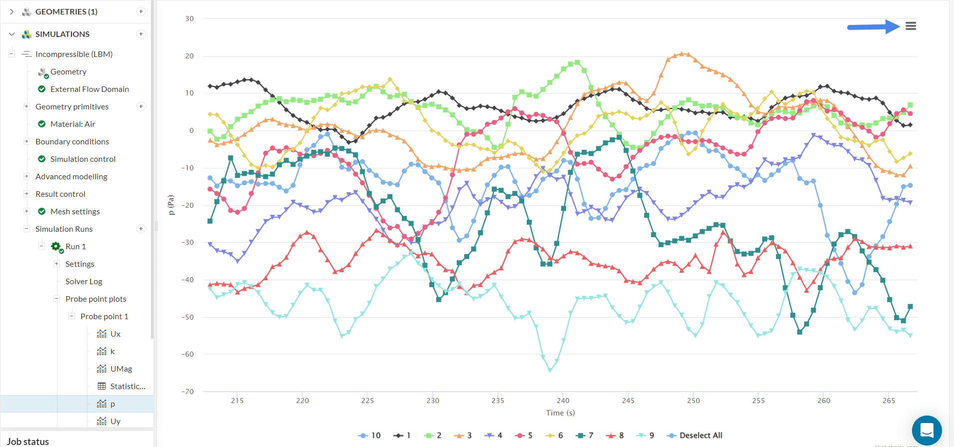
The results that are available for the defined probe points are:
- Pressure (p)
- The magnitude of Velocity (UMag)
- Velocity in x, y, and z-directions (Ux, Uy, and Uz respectively)
- Turbulent kinetic energy (k)
- Statistical data
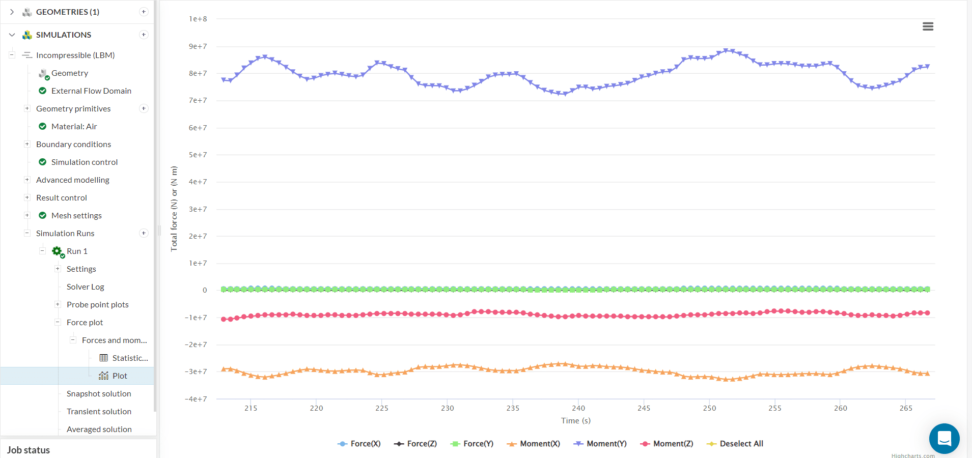
b. FORCE PLOT
Similar to the result of your probe points, the result of the forces and moments are also displayed in a temporal plot and a statistical summary. The forces and moments are calculated individually in the x-, y- and z-direction.
This tutorial shows how effectively the Incompressible LBM analysis type performs for external aerodynamics around a large city block. In conjunction with the Pedestrian Wind Comfort analysis type, you can propose better designs and ensure the safety of pedestrians.
Congratulations! You finished the wind analysis tutorial!
Note
If you have questions or suggestions, please reach out either via the forum or contact us directly.
References
Last updated: September 25th, 2023
Did this article solve your issue?
How can we do better?
We appreciate and value your feedback.


