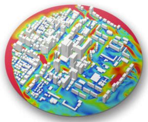
Incompressible Fluid Flow (LBM) analysis type is used to simulate the transient effects of external flow around objects using the Pacefish®\(^1\) Lattice Boltzmann method (LBM). This article answers the following questions regarding the simulation time and timestep in LBM Analysis:
- Can I control simulation time in LBM?
- Is it possible to control the simulation timestep in LBM?
Solution
The short answer is,
- Yes, you can control the simulation time
- No, you cannot control the timestep
1. Simulation Time
LBM is a transient (time-dependent) analysis. In other words, LBM analysis captures the transient behavior of the flow. In a time-dependent analysis, simulation time defines how long a transient simulation runs in terms of time (counted in seconds).
How long should be the simulation time? You can define the simulation time with respect to the number of fluid passes.
1.1 Number of Fluid Passes
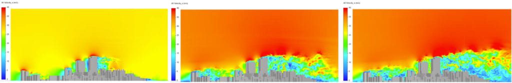
In transient flow analysis, initial time steps are unsteady. During the initial stage, it is assumed that first fluid particles enter the domain, then leave it. After that, the next party comes and leaves the domain. During the early fluid passes, we expect the flow to get developed. We assume that flow reaches a steady-state in the final fluid pass. As a result, we can say that 3 fluid passes are sufficient to reach the developed flow. In conclusion, the number of fluid pass defines the simulation time.
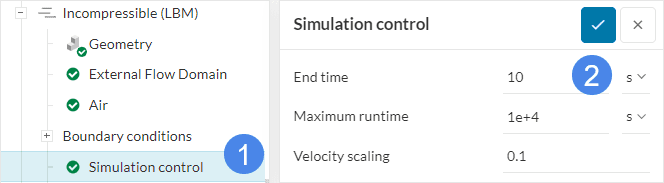
1.2 How to Define Simulation Time
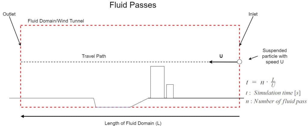
Calculate how long does it take a fluid particle to pass though the domain:
$$t_1 = \frac{L}{U} \tag{1}$$
where, \(t_1\) is the time requirement for 1 fluid pass, \(L\) is the length of fluid domain, and \(U\) is the speed of particle.
Multiply the number of fluid passes to find the total simulation time:
$$t_{total} = n\cdot \frac{L}{U} \tag{2}$$
where, \(t_{total}\) is the simulation time, and \(n\) is the number of fluid passes.
2. Simulation Timestep
Simulation timestep is the small-time intervals in a transient simulation. The user has no control over the timestep because a special algorithm in the LBM solver calculates the simulation timestep automatically.
Best Practices
Consider minimum 3 fluid passes in order to define the simulation time.
Related Articles
A similar concept is applied to control simulation parameters for pedestrian wind comfort simulations. Have a look at the following article to know more about fluid passes and maximum run time: https://www.simscale.com/knowledge-base/time-step-transient-lbm/
- Simulation Control for Wind Comfort
- How to Determine the Time Step Size for Transient Output in LBM Simulations?
Note
If none of the above suggestions solved your problem, then please post the issue on our forum or contact us.
References


