Tutorial: LBM Simulation of a Truck’s Aerodynamics
This tutorial is a step-by-step guide on setting up and running an external aerodynamics simulation around a truck using the Incompressible Lattice-Boltzmann solver\(^1\). Note that this solver is accessible on-demand, for professional users only.
Note
This tutorial uses the Lattice Boltzmann method (LBM), provided by Numeric Systems GmbH (Pacefish®)\(^1\), to run the simulation. This solver is only accessible through professional licenses, therefore this tutorial cannot be performed using a community license – Learn more about SimScale’s professional license options.
If you want to perform external aerodynamics with a community license, please check out
this tutorial.
Overview
This tutorial teaches, using a truck model, how to:
- Set up and run an LBM-Lattice Boltzmann method simulation
- Assign Geometry primitives in SimScale
- Assign boundary conditions, material, and other properties to the simulation
- Mesh with the SimScale LBM manual mesher.
We are following the typical SimScale workflow:
- Setting up the simulation
- Creating the mesh
- Running the simulation and analyzing the results
1. Prepare the CAD Model and Select the Analysis Type
As a first step, click on the button below. It will copy the tutorial project containing the geometry into your Workbench.
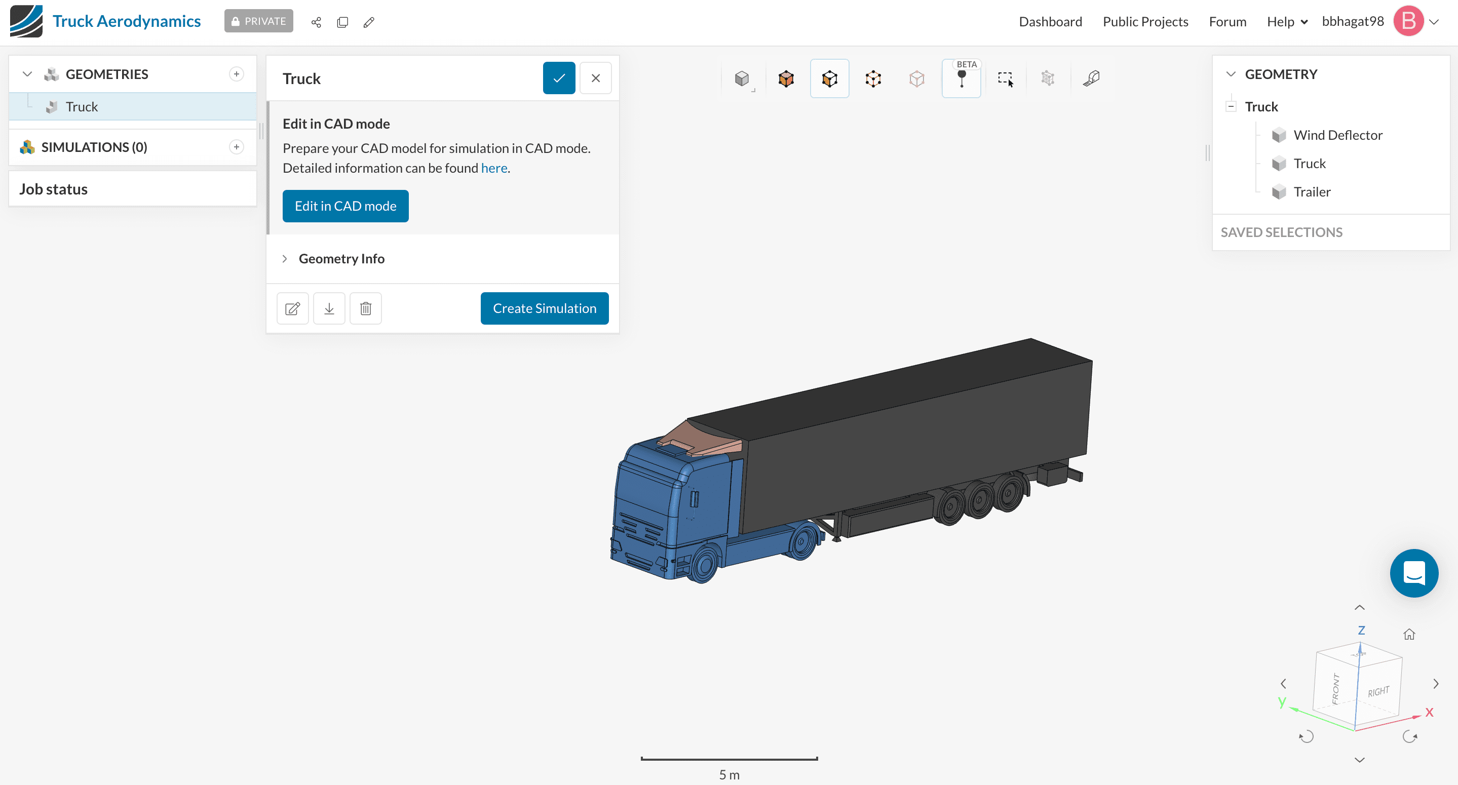
The following picture demonstrates what is visible after importing the tutorial project.
1.1 Create the Simulation
Before setting a simulation to run, we need to select the analysis type of interest:
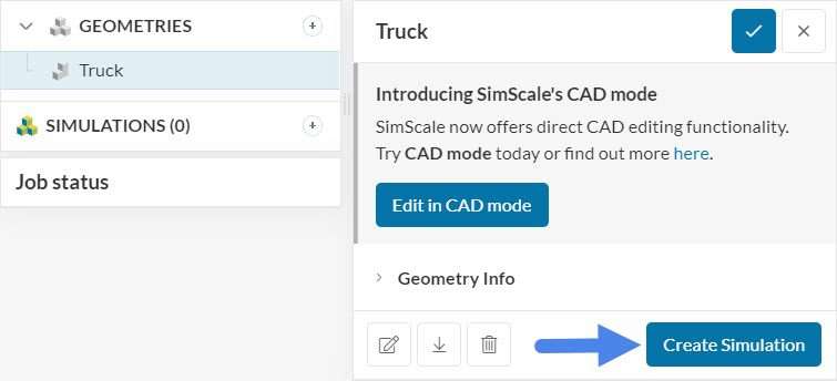
After clicking on the ‘Create Simulation’ button, the analysis type widget appears:
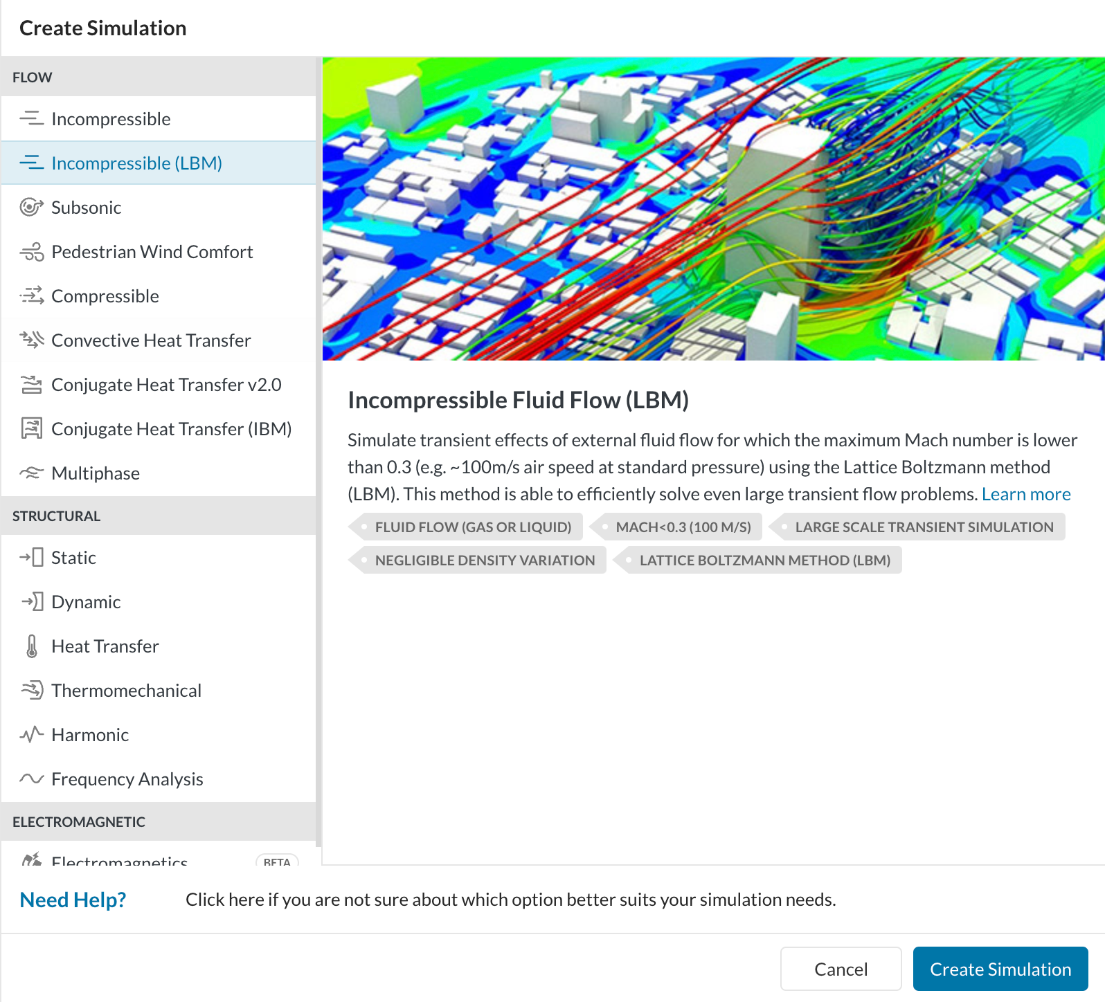
The Incompressible (LBM) solver is a powerful external aerodynamics module that runs in GPUs. This solver is transient by nature and allows fast computing times even for large grids. Please visit this page for more details on the Incompressible (LBM) solver.
At this point, a new simulation tree loads in the Workbench. In the global settings, we have multiple turbulence models to choose from
For this simulation, the default turbulence model (‘k-omega SST DDES’) is used – more details about this and other turbulence models are available here.
1.2 External Flow Domain
In this simulation type, one of the most important settings is the External flow domain dimensions. Here the user can define a cartesian box that represents the computational domain. It is important to make the cartesian box large enough, preventing negative impacts of the boundary conditions on the region of interest.
Below, you will find a rule-of-thumb that can be used as a starting point. The dimensions are based on the length L of the truck, which is roughly 16 meters in this model.
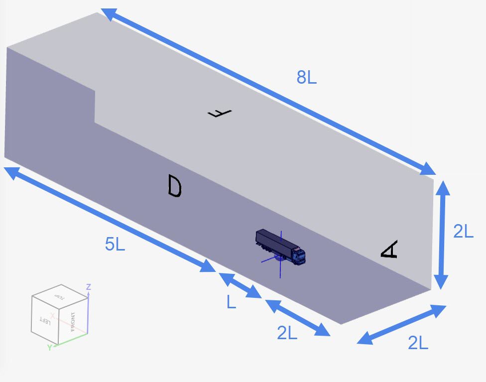
Notice how the flow domain is longer downstream from the truck: this is mostly to allow the wake to develop. Following the rule-of-thumb above, we will obtain the coordinates in Figure 7:
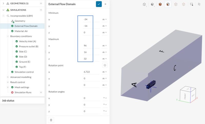
- x min: ‘-34’ \(m\)
- y min: ‘-16’ \(m\)
- z min: ‘0’ \(m\)
- x max: ‘96’ \(m\)
- y max: ‘16’ \(m\)
- z max: ‘32’ \(m\)
Did you know?
By adjusting the Rotation angle of the external flow domain, it is possible to rotate the computational domain.
This feature is especially useful for yaw angle studies, as it swiftly rotates the domain without adjustments in the CAD model.
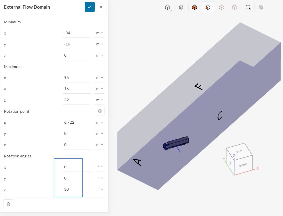
For this tutorial, all Rotation angles will remain at zero.
2. Assigning the Material and Boundary Conditions
In this section, we will define the physics of the simulation.
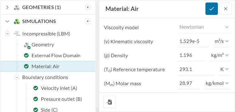
2.1. Define a Material
In LBM simulations, the solver automatically sets Air to the flow domain. However, it is possible to change the values of each field.
2.2. Assign the Boundary Conditions
As soon as an incompressible LBM simulation is created, the flow domain boundaries receive a set of default boundary conditions. For the default set of boundary conditions, the LBM solver makes the following assumptions:
- The positive z-direction is the sky;
- Without rotating the flow domain, the air flows in the positive x-direction, which represents the north.
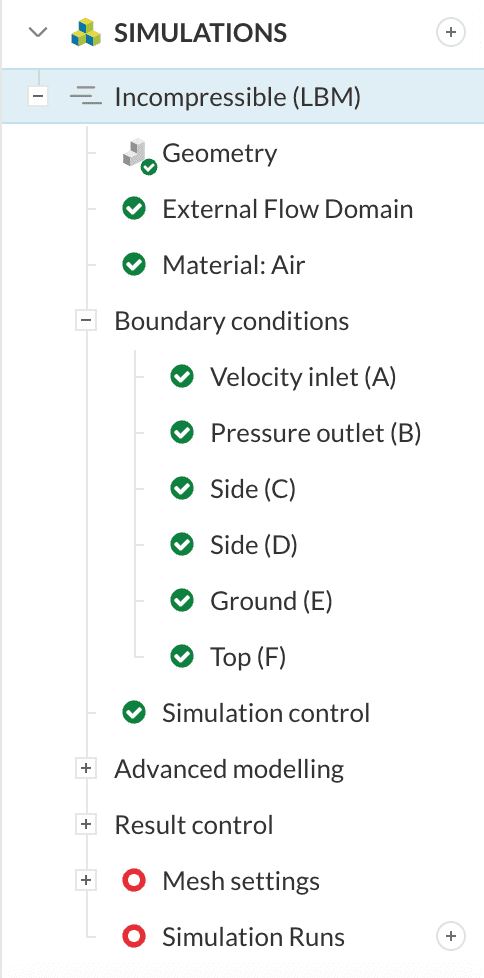
Since the CAD model from this tutorial follows the principles above, there are only a couple of adjustments needed from the default boundary conditions. The image below shows the boundary conditions used in this tutorial:
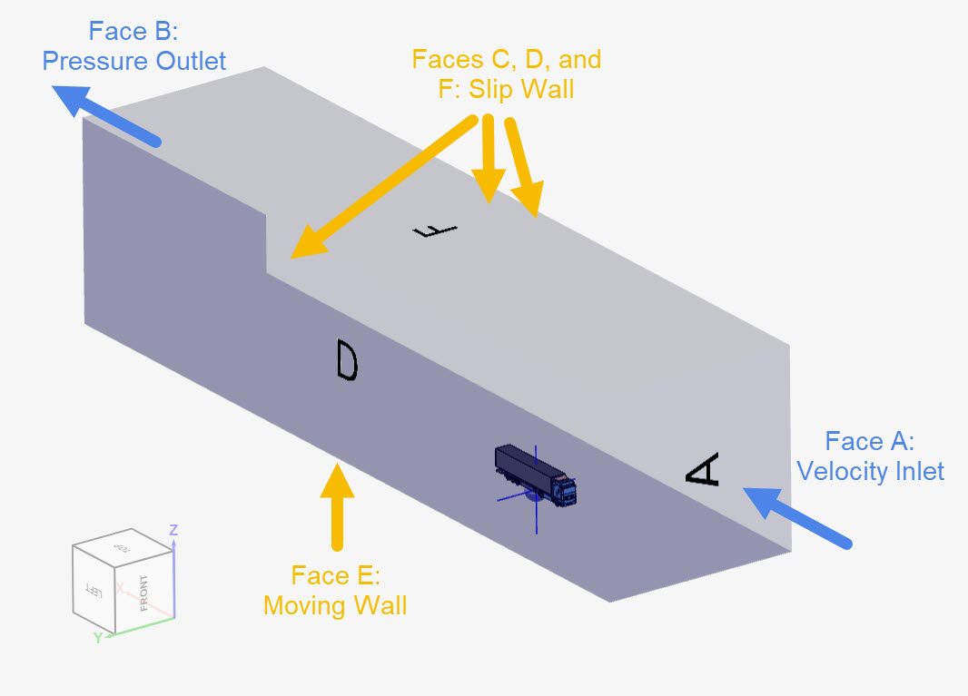
In this case, only two boundary conditions need adjustments: faces A and E.
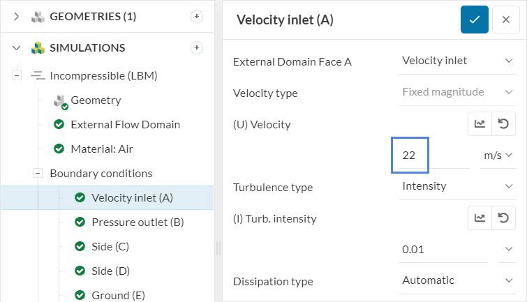
a. Velocity Inlet (A)
For the velocity settings, the user can define the velocity and turbulence. Please adjust the velocity to a fixed value of ’22’ \(m/s\).
Did you know?
You can upload a .csv file to define an atmospheric boundary layer profile for velocity and turbulence intensity/turbulent kinetic energy as a function of height. This is discussed in greater detail in the following post: Defining an Atmospheric Boundary Layer.
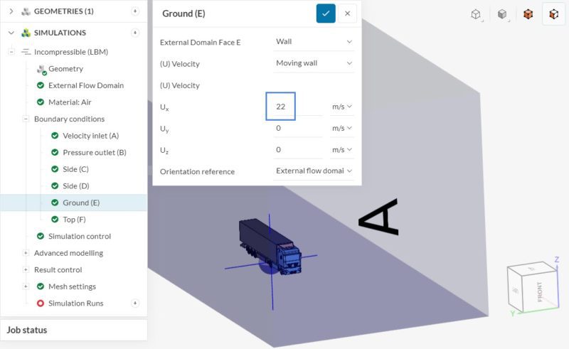
b. Ground (E)
By default, the ground face receives a No-slip condition, which is adequate for simulations with standing objects. Since the truck is moving, we will adjust the ground to ‘Moving wall’, with the same value as the velocity inlet in the positive x-direction:
2.3. Simulation Control
Under Simulation control, we can adjust the End time of the simulation. As a rule of thumb, we should ensure at least 2 fluid passes through the computational domain – this means that a particle should have time to flow from inlet to outlet at least 2 times during the simulation.
Referring back to Figure 7, the flow domain has 130 meters in the x-direction, and we have a velocity of 22 \(m/s\) at the inlet. This means that we need at least 11.82 seconds for the end time of the simulation. In this tutorial, we will use an End time of ’15’ seconds.
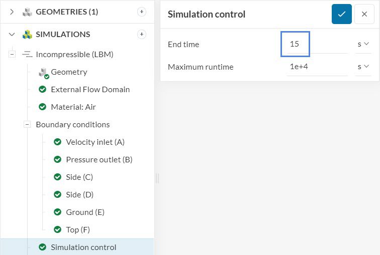
The Maximum runtime represents the wall-clock time that the simulation is allowed to run for. For this simulation, the default setting of 10000 seconds works very well.
2.4. Advanced Modelling
Under the Advanced modelling section, you will find additional physics to use, such as Rotating walls and Porous objects. The truck has five sets of wheels that act as rotating walls.
For the set up of a rotating wall, the user defines the Axis of rotation, a point on the axis of rotation (Origin), and the Rotational velocity. As a result, one rotating wall configuration is needed for each set of wheels.
Find below the steps for the first set of wheels of the truck:
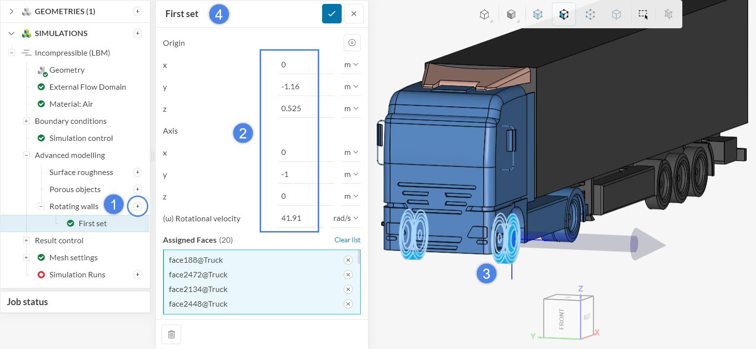
- Create a new rotating wall by clicking on the ‘+’ button next to Rotating walls. This will open a settings panel to define the Origin, Axis, and Rotational velocity.
- In order to identify the origin of the axis, select one of the faces of the first set of wheels
- Now click on the ‘Pick Center of current selection’ option. This will set the origin.
- The wheels rotate around negative Y axis. Change the y value for the Axis of rotation to ‘-1’. The settings below are good for the first set of wheels:
- Origin:
- x: ‘0’ \(m\)
- y: ‘-1.21’ \(m\)
- z: ‘0.525’ \(m\)
- Axis:
- x: ‘0’
- y: ‘-1’
- z: ‘0’
- Rotational velocity: Please note that the right-hand rule applies to the direction of rotation. To calculate the rotational velocity, we can use \(V = \omega r\), where \(V\) is the linear velocity of the truck, and \(r\) is the radius of the wheel. The resulting rotational velocity is ‘41.91’ \(rad/s\).
- Origin:
- Complete the definition by selecting the box ‘Assigned faces’ and adding all 20 faces from the first row of wheels.
- If you would like, you can change the name of the rotating wheel window to a more fitting one, for example, ‘First set’.
- Create a new rotating wall by clicking on the ‘+’ button
- Assign the 20 faces from the first row of wheels
- If you would like, you can change the name of the rotating wheel window to a more fitting one, for example, ‘First set’.
Now, repeat the same process for the other 4 sets of wheels. The table below summarizes the settings:
| Set | Second set | Third set | Fourth set | Fifth set |
| Origin x (m) | 3.9 | 9.794 | 10.944 | 12.094 |
| Origin y (m) | -1.15990381 | -1.15990381 | -1.15990381 | -1.15990381 |
| Origin z (m) | 0.525 | 0.525 | 0.525 | 0.525 |
| Axis x | 0 | 0 | 0 | 0 |
| Axis y | -1 | -1 | -1 | -1 |
| Axis z | 0 | 0 | 0 | 0 |
| Rotational Velocity (rad/s) | 41.91 | 41.91 | 41.91 | 41.91 |
| Number of faces for the assignment | 32 | 26 | 26 | 26 |
Coordinates of origin for different wheel sets
Since all wheels are located at the same height the z-coordinate will be same for all sets of wheels.
All wheels rotate about the negative y axis, hence, y-coordinate can be anything as long as the x- and z-coordinate match the values mentioned in Table 1.
Only the x-coordinate of the origin will change for different sets of wheels.
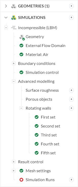
Once you finish this process for all sets, you should have this list on your simulation tree:
2.5. Result Control
The Result control settings allow us to define what information we want to obtain from the results. Several options are available, among forces and moments, probe points, vorticity, etc. – Please check this page for an overview.
In this tutorial, we will set up the Transient output, Statistical averaging, and Snapshot.
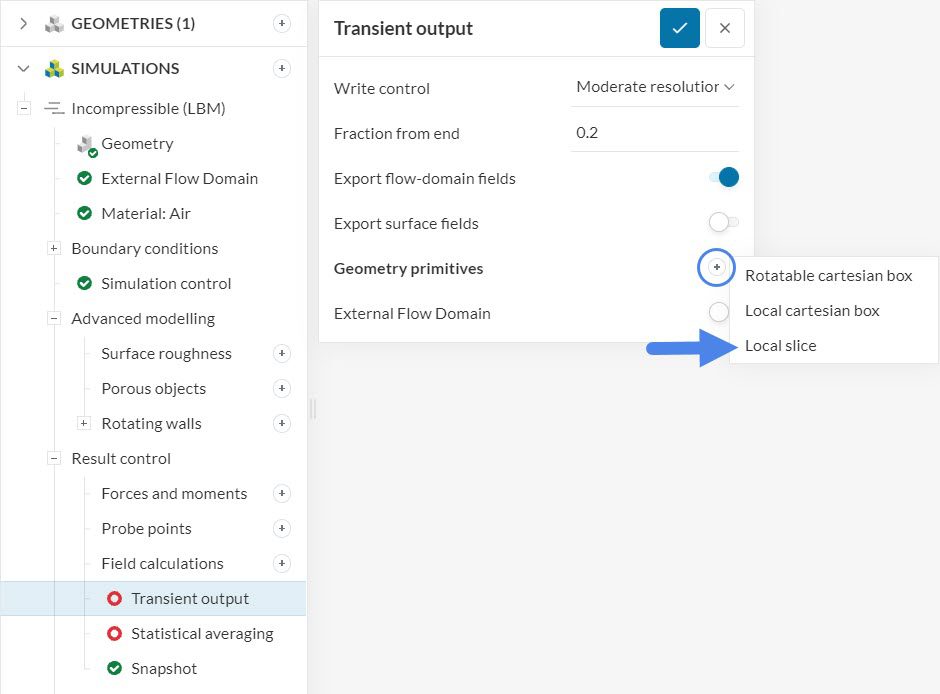
a. Transient Output
In short, the transient output consists of datasets extracted from the results at a certain frequency. For this tutorial, we will create a Local cartesian box and assign it to the transient output.
Care must be taken with the transient output, as it can generate several gigabytes of data if one is not cautious. A good practice is to use Local slices or a small Local cartesian box. For a full description of the transient output, please refer to this page.
After expanding Result control and selecting Transient output, please click on the ‘+’ button next to Geometry primitives and select a ‘Local slice’:
In the window that pops up, adjust the Normal to the y-direction:
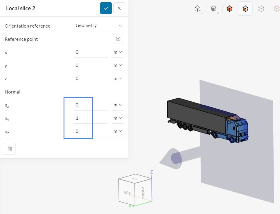
After saving the local slice settings, it will automatically be assigned to the transient output. Before saving the settings, enable ‘Export surface fields’ and select the three parts of the model in the geometry tree on the right (Trailer, Truck and Wind Deflector). This option will save the transient results on the walls of the truck as well.
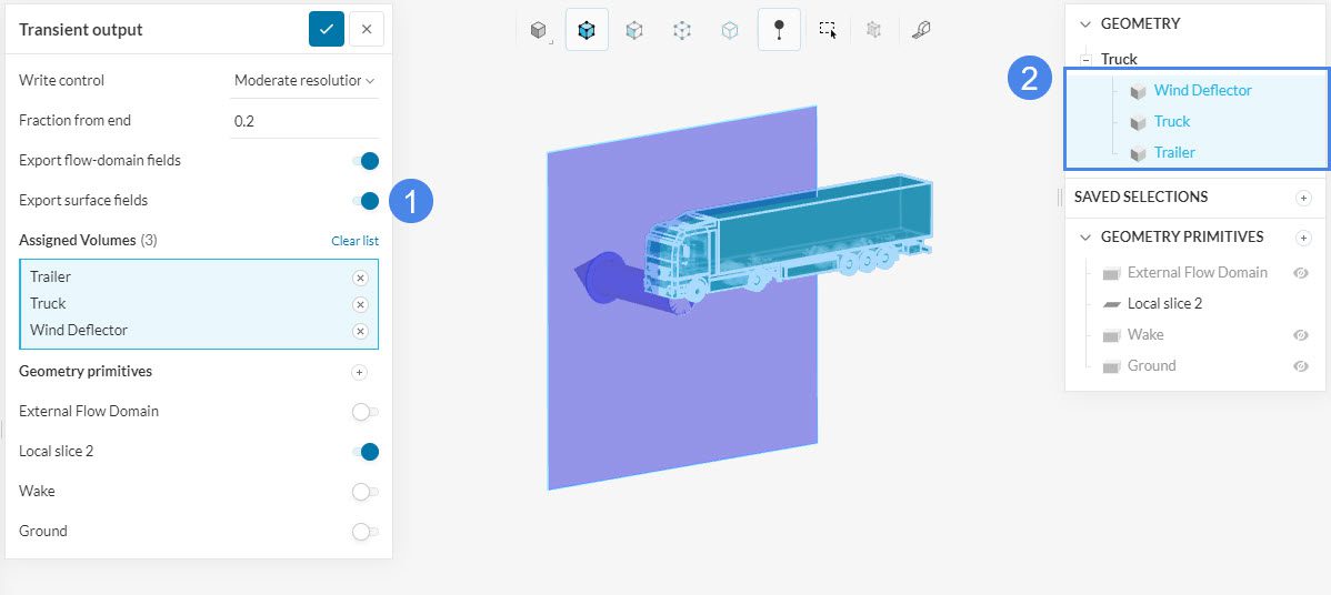
With a Fraction from end of 0.2, this result control will start saving data in the final 20% of the simulation, with a moderate frequency.
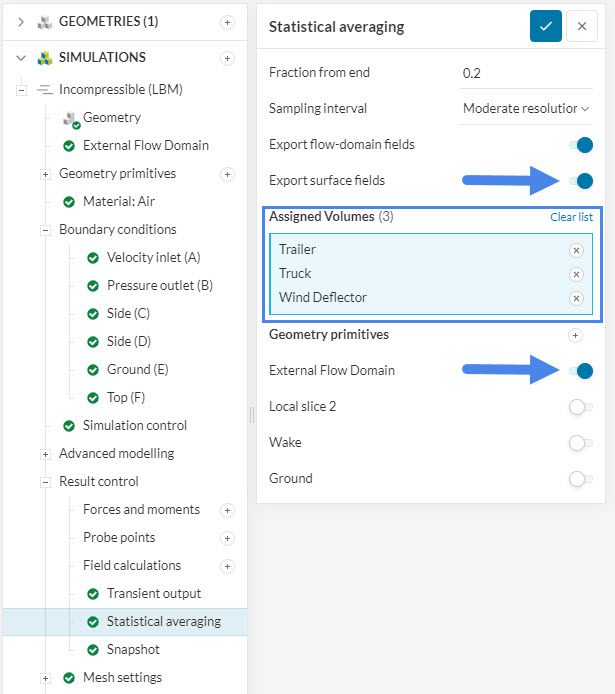
b. Statistical Averaging
To obtain the mean values from the transient simulation we use the Statistical averaging result control. The statistical results are less memory-intensive than the transient output, so we can use larger geometry primitives, if necessary. Please assign the ‘External Flow Domain’ to the Statistical averaging output, enable the ‘Export surface fields’ option and select the three volumes of the truck in the assignment box as already done for the transient output.
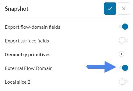
c. Snapshot
The result control item Snapshot saves the data from the final time step of the simulation. In this case, please assign the ‘External Flow Domain’ volume to it:
3. Mesh Settings
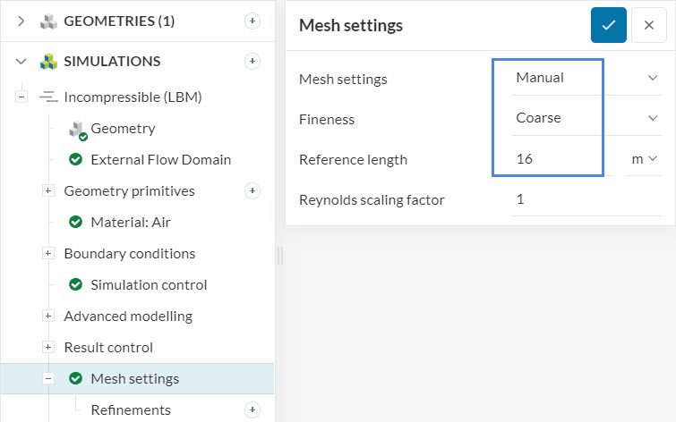
The Incompressible LBM analysis allows automatic and manual meshing. For an in depth description of the mesh settings, please visit this documentation page.
In this tutorial, we will make use of the ‘Manual’ configuration, using a ‘Coarse’ fineness. The Reference length represents the longest characteristic length of the geometry – for a truck, the length of the vehicle is the best choice.
3.1. Meshing Refinements
This meshing tool also allows refinements for a better mesh resolution within the regions of interest.
a. Region Refinements
A region refinement allows you to control the maximum cell size in a certain region of the domain. Follow the steps below to create a region refinement:
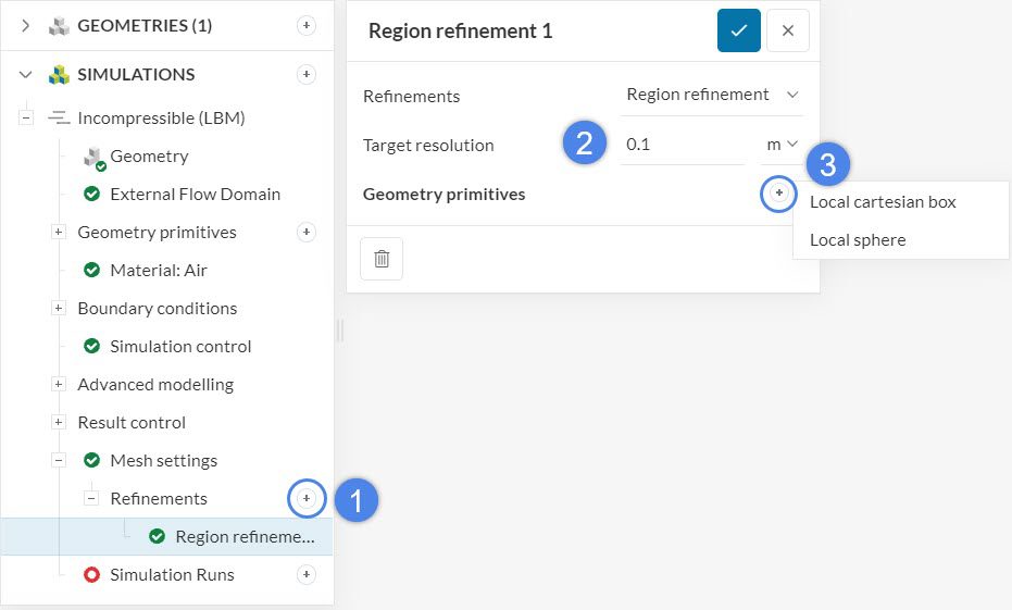
- Click on the ‘+’ button next to Refinements. From the list, select a ‘Region refinement’
- Based on the Target resolution, the meshing tool will control the local cell size so it won’t be larger than this value. Please adjust the Target resolution to ‘0.1’ \(m\)
- Click on the ‘+’ button next to Geometry primitives and select a ‘Local cartesian box’.
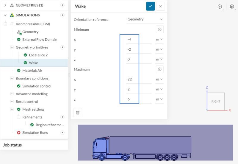
In the local cartesian box configuration window, type in the coordinates below:
After saving the settings, create a second Local cartesian box with the following coordinates:
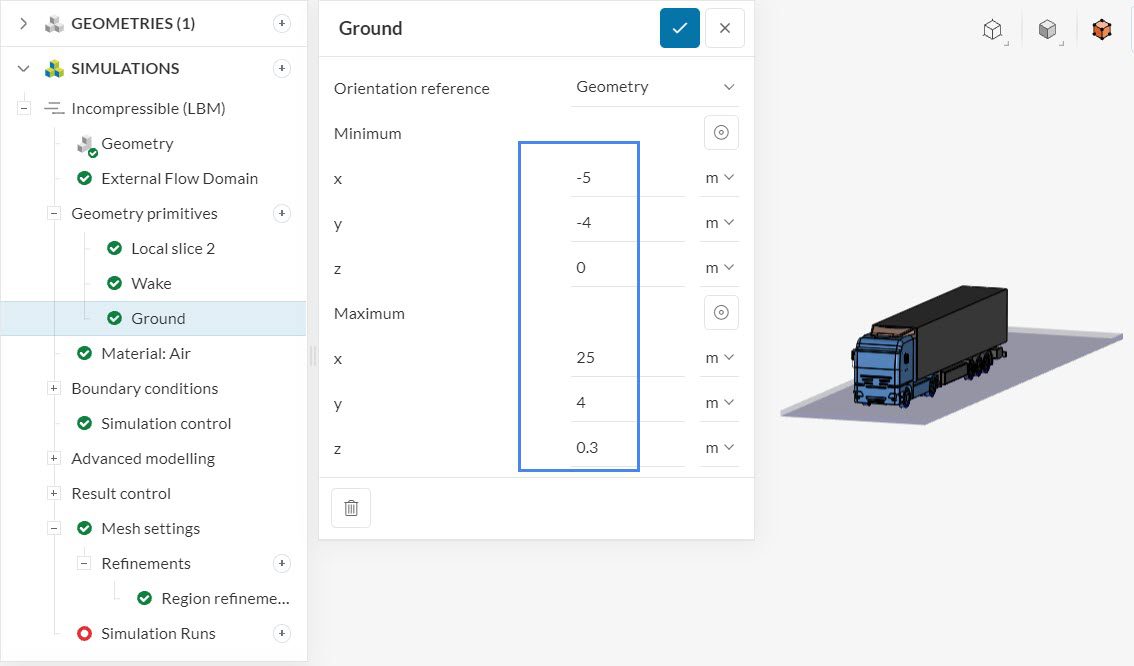
After saving, make sure that both local cartesian boxes are assigned to the region refinement.
b. Surface Refinement
The next refinement is a Surface refinement for the truck walls. The image below shows the steps:
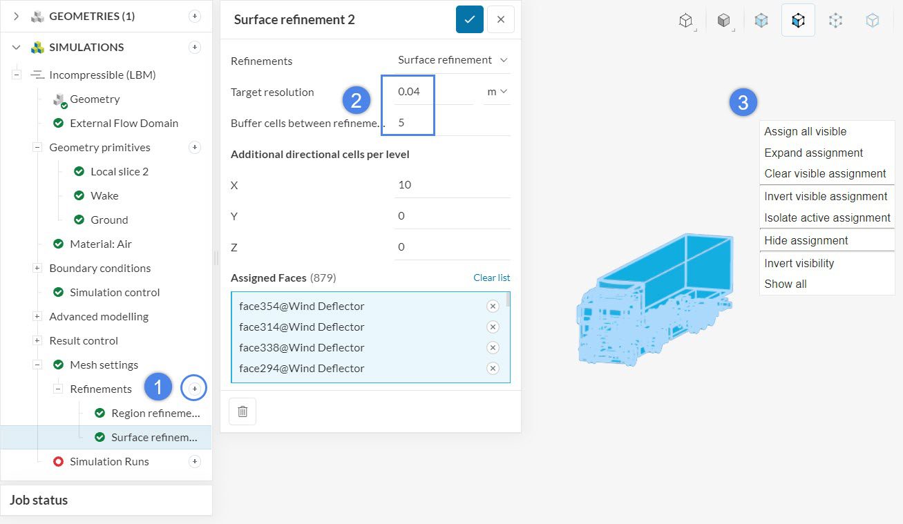
- After clicking on the ‘+’ button next to Refinements, select a ‘Surface refinement’
- Set ‘0.04’ \(m\) to the Target resolution, which is a good starting point for a truck. Furthermore, increase the Buffer cells between refinement levels to ‘5’
- The easiest way to assign all truck faces at once is by right-clicking and choosing ‘Assign all visible’
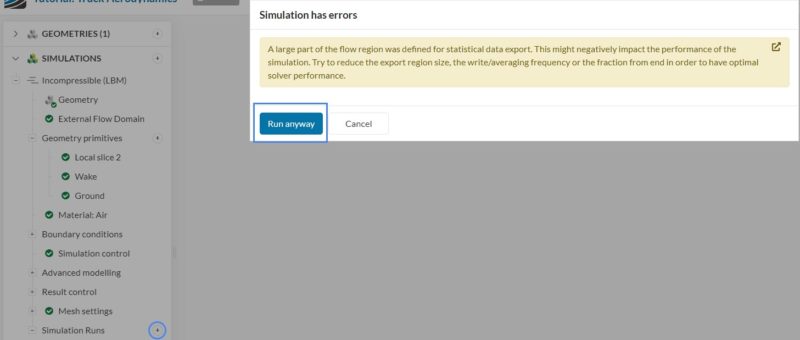
4. Simulation and Results
You are now able to start a simulation run by clicking on the ‘+’ button next to Simulation Runs. Please note that a warning message will show up – the warning message will not be an issue for this tutorial, therefore, select ‘Run anyway’.
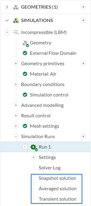
4.1 Post-Process the Results
After the aerodynamic analysis of the truck simulation has finished, you will have three main results at your disposal:
- Snapshot Solution: the result of the last timestep.
- Averaged Solution: an averaged result, with a sample of the last 20% of the simulation
- Transient Solution: a transient result based on the interval of the timesteps. Transient results can be animated as they contain data from several timesteps.
You can access these results under the simulation run, by clicking on the respective name:
As a demonstration, we will inspect the ‘Transient solution’ of this simulation. After opening the results, you will find the filters ribbon on the top, and the timestep selector on the right-hand side panel:
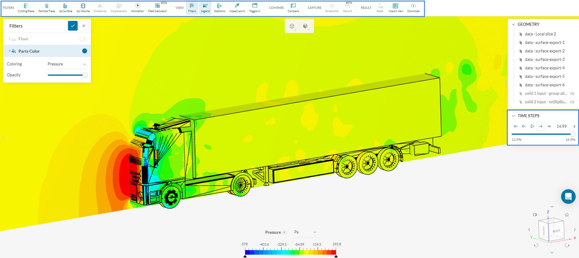
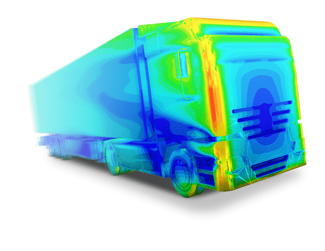
The timestep selector is particularly useful for transient runs, as you can go through the various saved states. In the Parts Color tab, under Coloring, it is also possible to choose a parameter to plot in the results. The image above is showing the pressure contours, however other parameters such as velocity are also available.
By selecting an ‘Animation’ filter from the top ribbon, we can create an animation over the timesteps from the results:
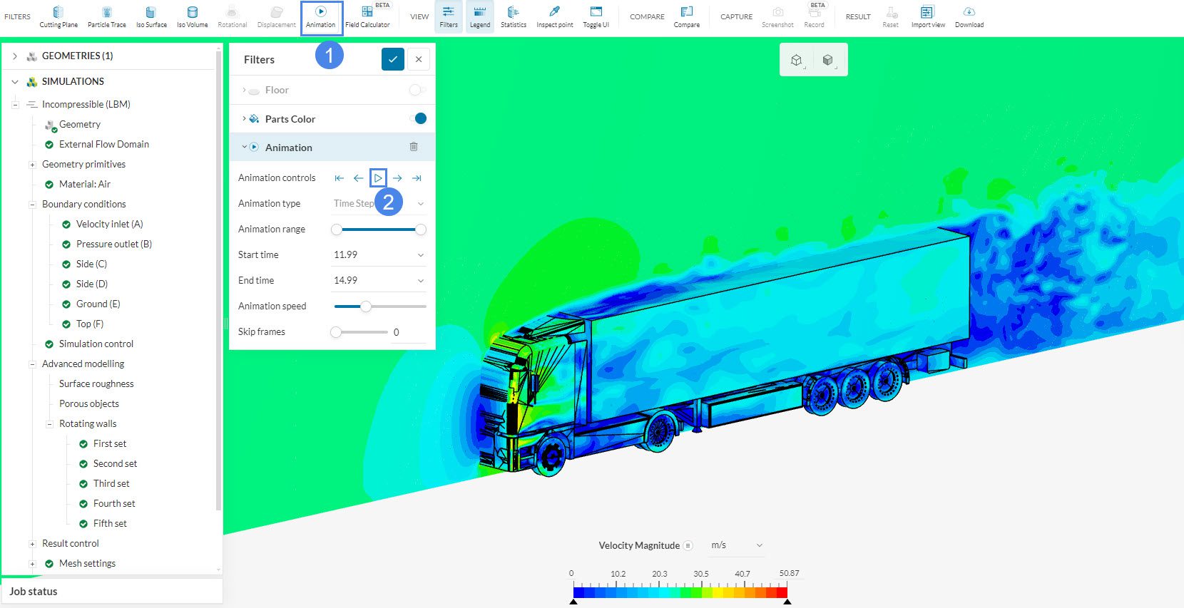
After pressing, the animation loads and you will see the results directly in the SimScale platform.
In conclusion, the Incompressible LBM analysis type is a powerful tool for transient external aerodynamics studies. It allows for quick simulation set ups, while maintaining robustness and speed as the simulation runs.
Congratulations! You finished the aerodynamic analysis of a truck tutorial!
Note
If you have questions or suggestions, please reach out either via the forum or contact us directly.
References
Last updated: February 15th, 2024
Did this article solve your issue?
How can we do better?
We appreciate and value your feedback.


