What is the Boussinesq Approximation?
The Boussinesq approximation is used to solve buoyancy-driven flows and is less computationally expensive than solving the full compressible formulation of the Navier-Stokes equations. The Boussinesq approximation can be used in all non-isothermal flows and ignores density differences except for equation terms which are multiplied by gravity.
By doing so, density differences due to inertial effects are completely ignored, and density is solely a function of temperature. The Boussinesq approximation assumes a constant kinematic viscosity and can be used for both turbulent and laminar flows.
The approximation assumes a linear change in density that is dependent on temperature. It is very accurate for natural convection flows at relatively low-temperature differences from ambient, where the Nusselt number is commonly used to characterize the resulting heat transfer. This makes it a good fit for relatively low-temperature electronics cooling, building HVAC, and thermal comfort. As flows become high speed (>120 m/s) or high temperature (> 100 °C), the approximation becomes less accurate as the linear assumption between temperature and density is no longer valid.
Boussinesq Approximation in CFD
The Boussinesq Approximation first gained popularity in the early days of computational fluid dynamics (CFD) because it reduces computational costs while still allowing a good density approximation. During the 1980s, when commercial CFD was still in its infancy, computing power was a small fraction of what it is today. By using the Boussinesq approximation, a moderate speed-up could be achieved.
As computational power has increased over the past several decades, the popularity of the Boussinesq approximation has become less relevant, yet it is still used in many commercial CFD codes today.
The Boussinesq Approximation Theory
While using the Boussinesq Approximation, density variations are a function of reference density, temperature, and a coefficient of thermal expansion.
$$ \rho = \rho_0 – \alpha \rho_0(T-T_0) $$
Where:
\(\rho\) = Local Density
\(\rho_0\) = Reference Density
\(\alpha\) = Coefficient of Thermal Expansion
\(T\) = Local Temperature
\(T_0\) = Reference Temperature
Boussinesq Approximation in SimScale
Within SimScale, we approximate air by using the following values:
\(\rho_0\) = 1.196 kg/m3
\(\alpha\) = 0.00343 1/K
\(T_0\) = 295.15 K
Therefore, we get:
$$ \rho = (1.196 kg/m^3) – (0.00343 1/k) * (1.196 kg/m^3) * (T-295.15 K) $$
Density using the Boussinesq approximation can be plotted as a function of temperature and compared against actual density in order to understand the correlation at common temperature ranges.
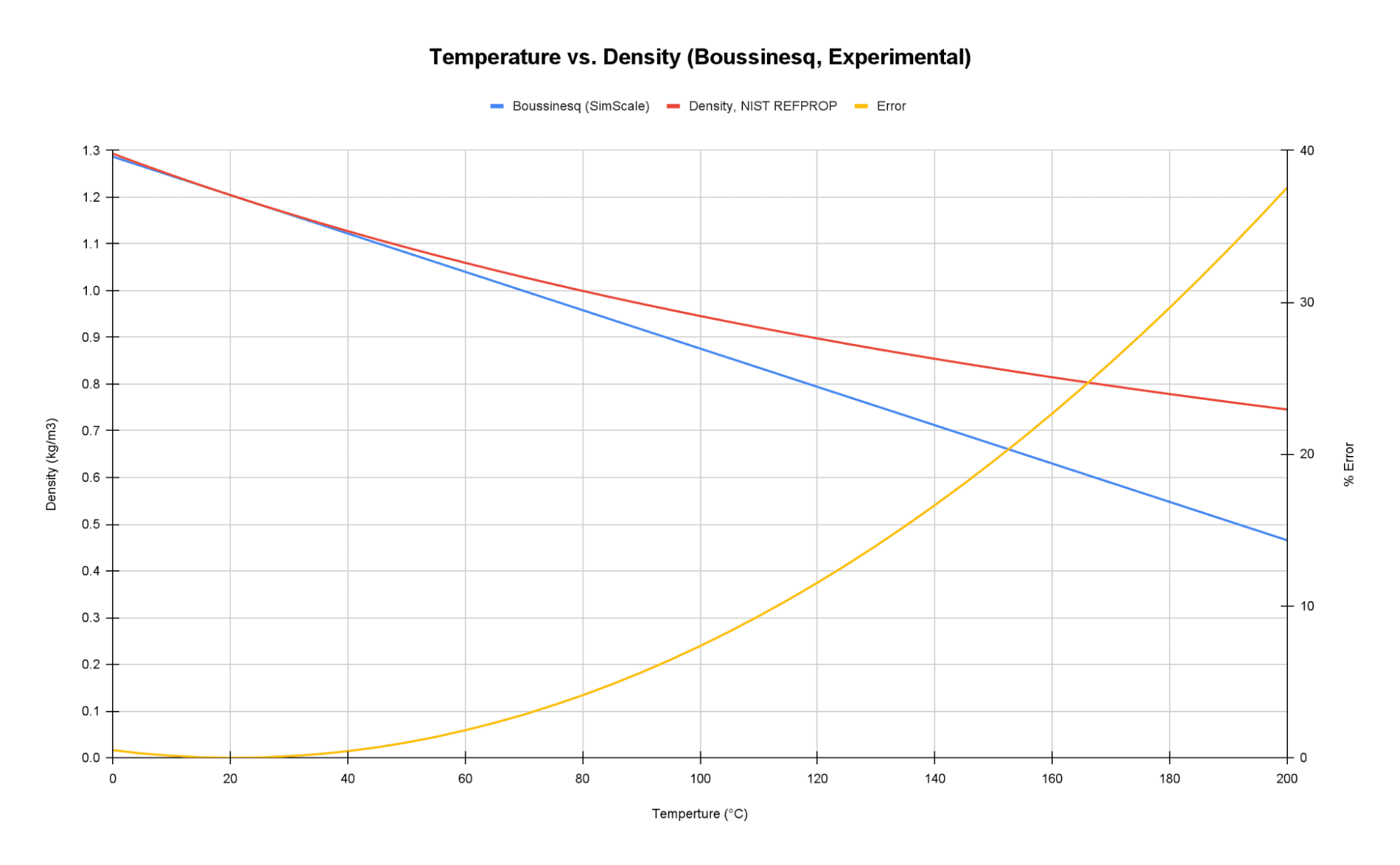
We can see the error between experimental air density and Boussinesq approximation density is less than 10% until ~ 115 °C. For SimScale conjugate heat transfer simulations that may have temperatures greater than 115 °C, it is recommended to turn on the Compressible flow option. By doing this, Air will be modeled as an ideal gas. The ideal gas law is valid for a much higher temperature and pressure range.
Example: Thermal Management of an Electronic Box
SimScale’s “Thermal Management of an Electronics Box” tutorial uses a fully compressible, ideal-gas definition of air. To understand how the Boussinesq approximation can affect results, the tutorial project can be rerun with a Compressible set-off. By doing this, the Boussinesq approximation of air will be used.
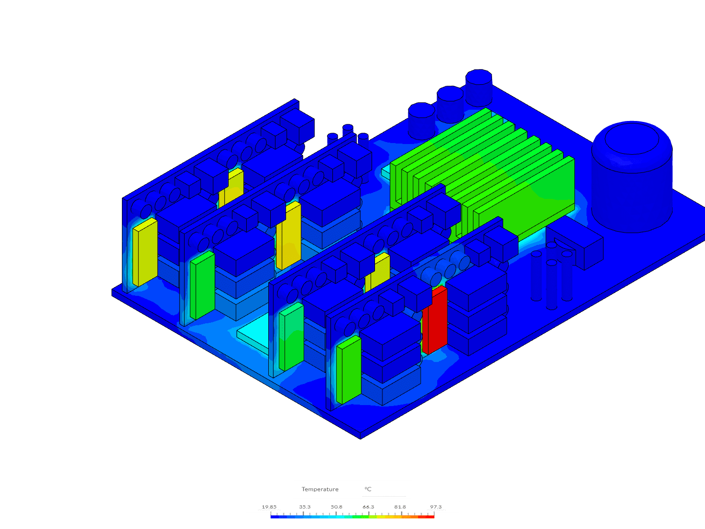
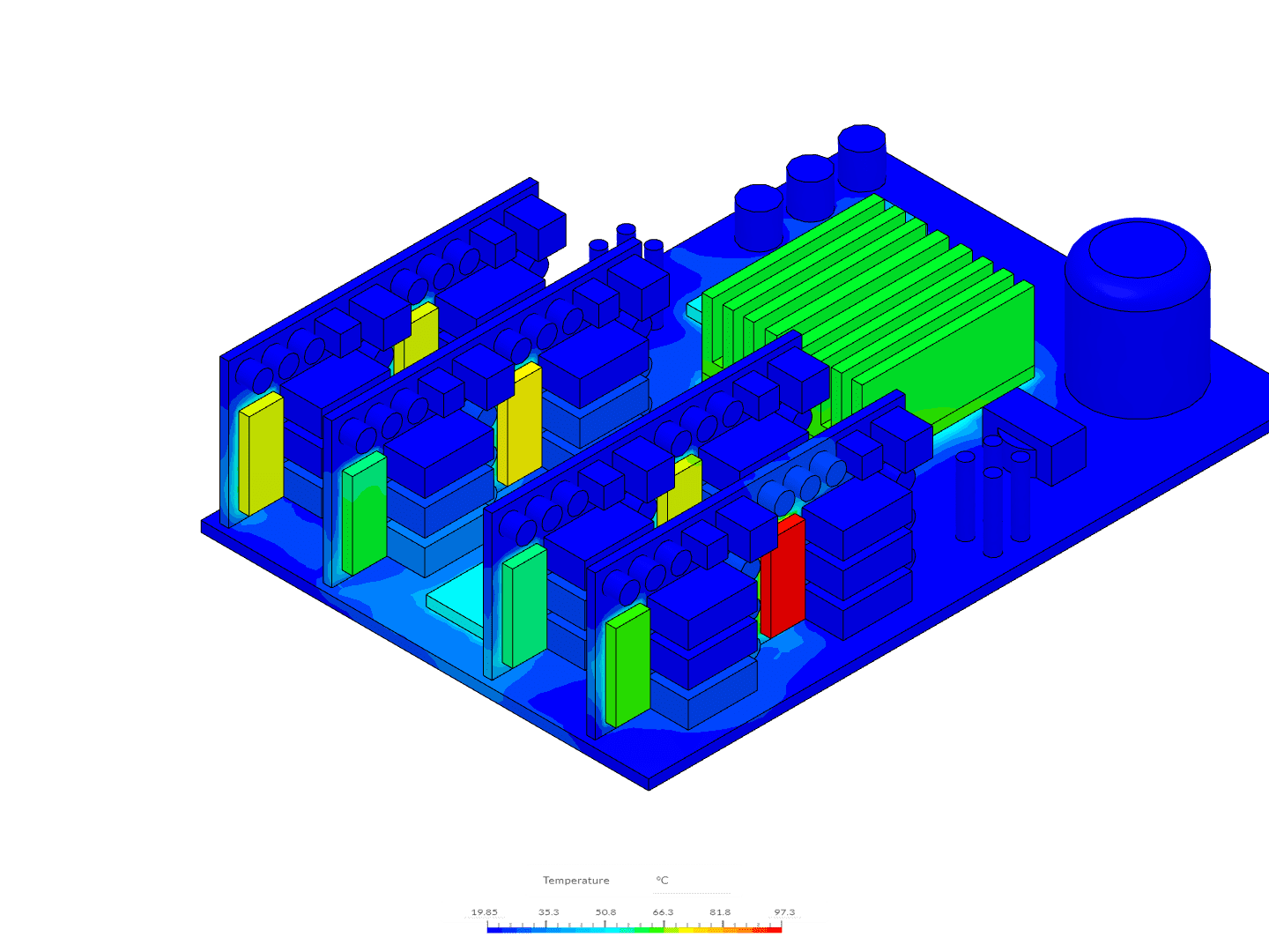
By comparing the results of the fully compressible run to the simulation using the Boussinesq approximation, we can see there is a negligible difference in results. The “Main Board Large Chip” has an average temperature of 59.6 °C using fully compressible and 58.6 °C with the Boussinesq approximation. Similarly, the maximum temperature in the domain is 97.3 °C using fully compressible, and 95.2 °C for the Boussinesq approximation.
Last updated: March 16th, 2026
Did this article solve your issue?
How can we do better?
We appreciate and value your feedback.
What's Next
The Lattice Boltzmann Method (LBM): A Comprehensive Guide

