Base Excitation
The Base excitation boundary condition allows to specify a base motion acceleration in a harmonic structural simulation. The acceleration is applied to all the faces that are constrained by means of a Fixed support boundary condition.
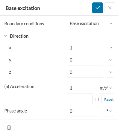
The parameters of the boundary condition to be defined are:
- Direction: Vector pointing in the direction of the initial acceleration. The vector is represented through its x, y, and z components in the global frame of reference.
- Acceleration: Scale factor for the acceleration vector, giving the magnitude of the acceleration. Can be specified as a constant value, or as a function of frequency using a table through the specify value button.
- Phase angle: Allows input of different loads that are not synchronized, or in other terms, when the peak value of the different loads do not occur at the same time. The value (\(\varphi\)) for the angle can be related to the excitation frequency (\(f\)) and the time delay between the peaks (\(\delta\)) of two loads:
$$ \varphi = 2 \pi f \delta $$
Important!
Notice that this boundary condition, unlike the other ones, does not contain an assignment panel. The base acceleration is applied to all the faces assigned to the Fixed support boundary condition or the Elastic support boundary condition but with a very high stiffness value.
Thus, it is necessary to first define the fixed (or high stiffness elastic supports) supports, then create the base excitation.
Supported Analysis Types
The following analysis types support the usage of this boundary condition:
Compatible Boundary Conditions
The Base excitation boundary condition can be used in combination, exclusively, with the following boundary conditions:
- (Another) Base excitation
- Fixed support
- Fixed value
- Symmetry plane
- Elastic support
- Bolt preload
- Point mass
This exclusivity implies that boundary conditions not listed above can not be used in combination with the base motion, and trying to do so will result in an error message.
Relative Frame of Reference
It is assumed that a rigid body motion is imposed to the fixed faces, due to the harmonic base excitation. Thus, the total displacement at any point in the structure can be expressed as the sum of a relative displacement with respect to the base and the rigid body motion of the base. The situation is illustrated in Figure 2:
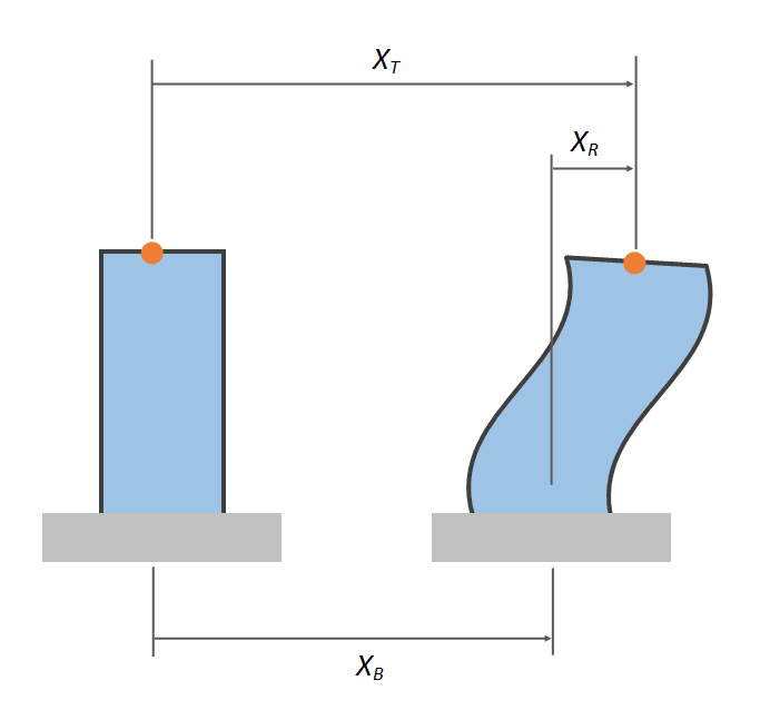
Analytically, this can be expressed as:
$$ X_T(t) = X_B(t) + X_R(t) $$
Which, due to the assumption of linearity in the harmonic analysis, also extends to the velocities and accelerations:
$$ \dot{X}_T(t) = \dot{X}_B(t) + \dot{X}_R(t) $$
$$ \ddot{X}_T(t) = \ddot{X}_B(t) + \ddot{X}_R(t) $$
In other words: one places the model in a frame of reference relative to the moving base, and the above corrections have to be performed in order to retrieve the motion with respect to an inertial frame of reference.
Moreover, all the displacements, velocities and accelerations in the result fields of a simulation under this boundary condition are expressed in the frame of reference relative to the base, and not in an inertial frame of reference. Thus, one has to be careful when comparing the results with other data, for example to experiments sampled with an accelerometer, where the registered values are total and not relative to the base motion.
Application Notes
This boundary condition is intended to evaluate the inertial effects of a structure subject to harmonic base motion, transmitted through the points of support. Some examples of such cases are:
- Shaker table testing
- Earthquake loads
- Base-induced vibrations
The effects of the inertial loads, developed due to the accelerated base motion, are evaluated in terms of the maximum quantities of interest, same as all steady state harmonic oscillations. That is, the results are expressed in terms of the peak displacement, stress and strains of the structure under the action of the base motion.
The option to scale the base acceleration magnitude as a function of the frequency allows to evaluate the response of the system against a known acceleration spectrum. The peaks in the response vs frequency graph, as measured with a Result control item – Point data, reveal which of the natural frequencies of the system are excited by the base motion, for the given direction of excitation.
To illustrate this, let’s have a look at the tip displacement of a cantilever beam under base excitation:
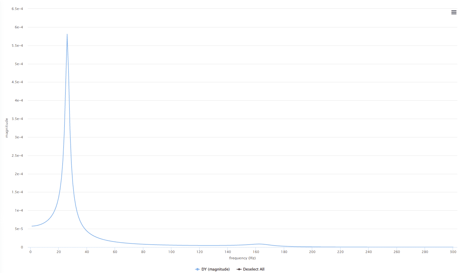
It can be seen from the figure, that one natural oscillation mode is excited by the base motion and resonance occurs, because of the peak in the frequency response graph. The location of the peak at 24 Hz also informs the value of natural frequency.
Related Documentation
- Fixed support boundary condition
- Harmonic analysis
- Validation case: Cantilever subject to base excitation
Last updated: March 5th, 2025
Did this article solve your issue?
How can we do better?
We appreciate and value your feedback.


