Advanced Tutorial: Natural Convection of a LED Spotlight
This tutorial shows how to perform a natural convection simulation on a LED spotlight, aiming to satisfy maximum temperature requirements and optimize LED performance.
This tutorial teaches how to:
- Set up and run a natural convection simulation using the Conjugate heat transfer solver;
- Assign boundary conditions, material, and other properties to the simulation;
- Mesh with the SimScale standard meshing algorithm.
We are following the typical SimScale workflow:
- Prepare the CAD model for the simulation.
- Set up the simulation.
- Create the mesh.
- Run the simulation and analyze the results.
Did you know?
For applications with LEDs, it’s important to control the temperatures developing on the chips. A poor design, with high temperatures, is harmful to the lifetime of a LED package.
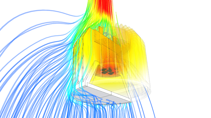
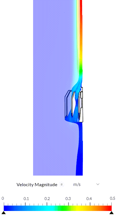
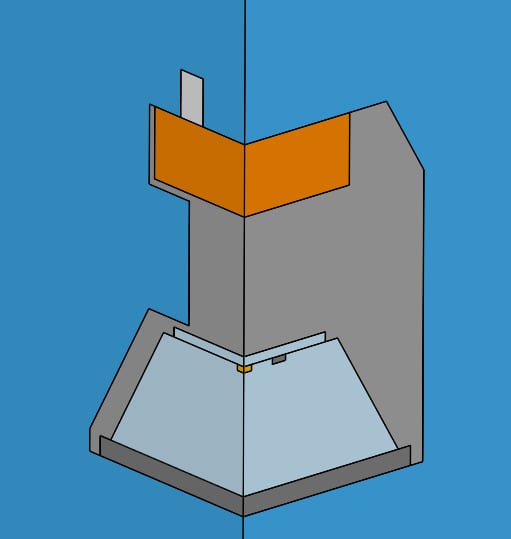
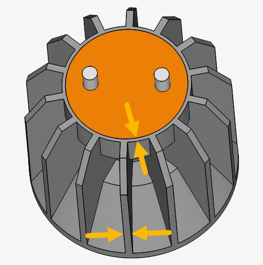
In this tutorial, we will simulate how effective natural convection is in cooling our geometry:
Learn with the video!
The following tutorial is also available in a video format with all steps described in equal details. Experience this interactive way of learning and let us know your thoughts in the comments section.
1. Prepare the CAD Model and Select the Analysis Type
As a first step, please click on the button below. It will import the tutorial project directly into your Workbench.
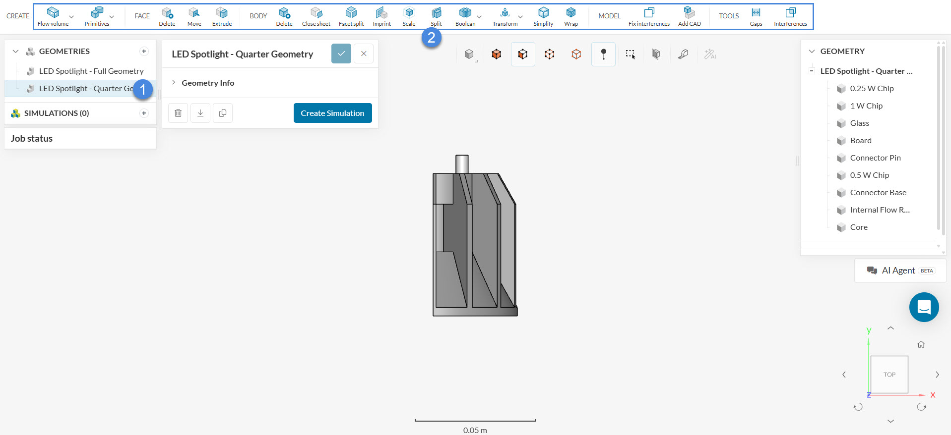
The following picture demonstrates what should be visible after importing the tutorial project:
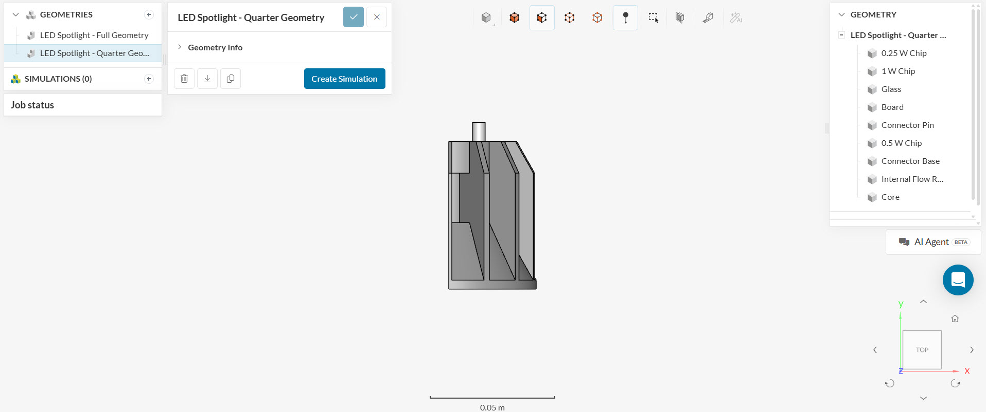
Note that the project contains two geometries. The first one consists of the complete LED spotlight geometry, and the second one consists of a 90 degrees slice.
Did you know?
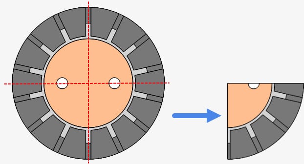
It’s possible to use the symmetrical nature of the LED spotlight geometry in our favor. Since we expect the flow to be mirrored along the symmetry planes, we can use just a quarter of the geometry. This brings a series of benefits, such as:
– Allows faster meshing operations and simulation runs
– Possibility to use finer cells, thus improving the domain discretization
1.1. CAD Edit
The initial CAD geometry only contains the LED spotlight parts. Before starting to work on the setup, we have to create the external flow volume, and also imprint the geometry.
The external flow region should be large enough to prevent the boundary conditions from interfering with the results. In Figure 5, you will find a good rule of thumb for the flow volume dimensions:
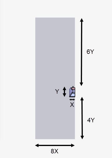
- Top: 6 times the height of the LED spotlight
- Bottom: 4 times the height of the geometry
- Sides: 8 times the width of the geometry
To perform the necessary operations, we are going to use the CAD environment. To modify a CAD model, simply select the geometry from the list—the available CAD operations will then appear in the top toolbar. You can either work directly on the original model or create a duplicate and apply your changes to the copy.
Once the editing begins, we can proceed to create an External Flow Region. Based on the rule of thumb presented in figure 5, we can set the minimum and maximum coordinates:
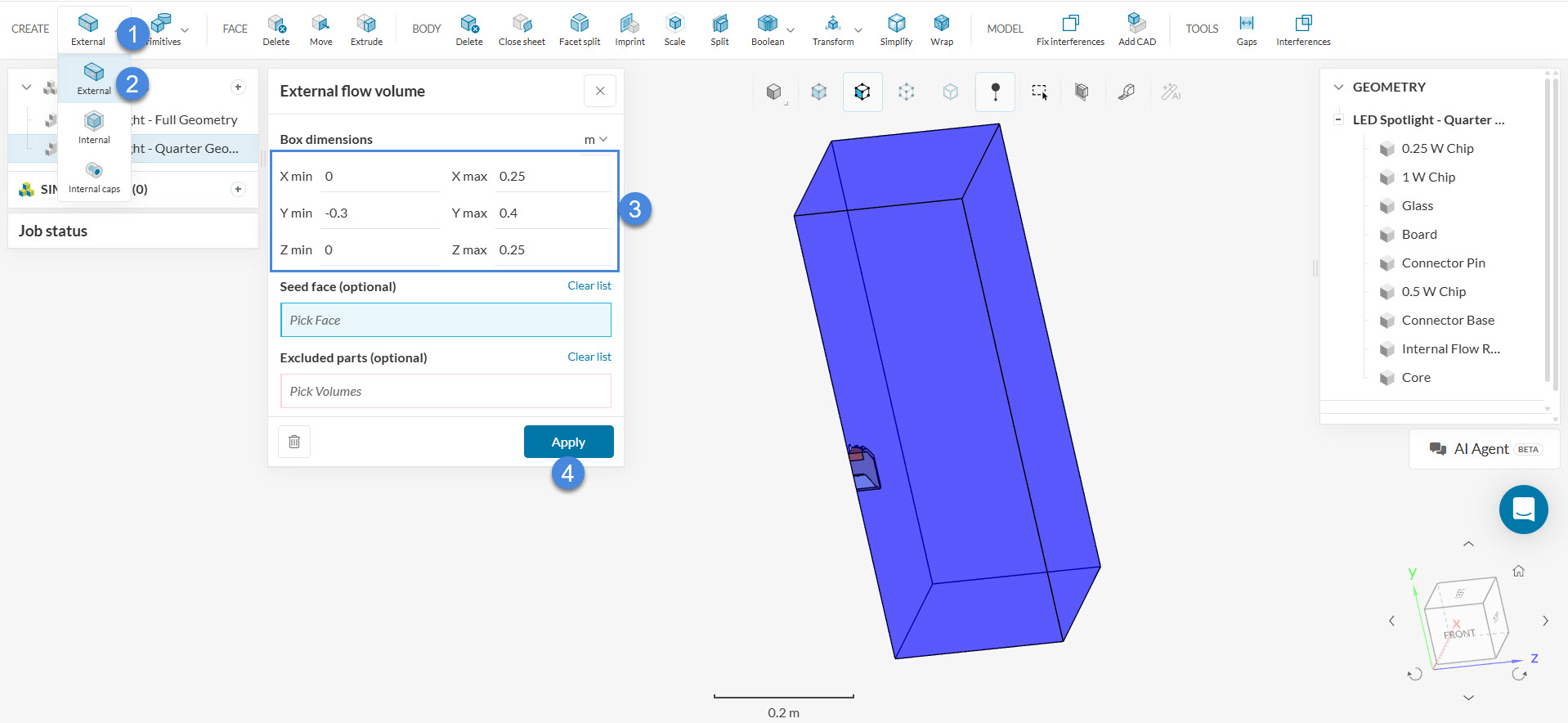
- Create an ‘External’ flow volume operation
- Set the flow volume dimensions to the following:
- X min value: ‘0’ meters
- Y min value: ‘-0.3’ meters
- Z min value: ‘0’ meters
- X max value: ‘0.25’ meters
- Y max value: ‘0.4’ meters
- Z max value: ‘0.25’ meters
- Hit ‘Apply’ to run the operation.
Another important step is to run an Imprint operation. In our LED geometry, a series of interfaces between solid/solid and solid/flow regions are present. The imprint operation improves the automatic detection of such interfaces.
Therefore, please follow the steps below:
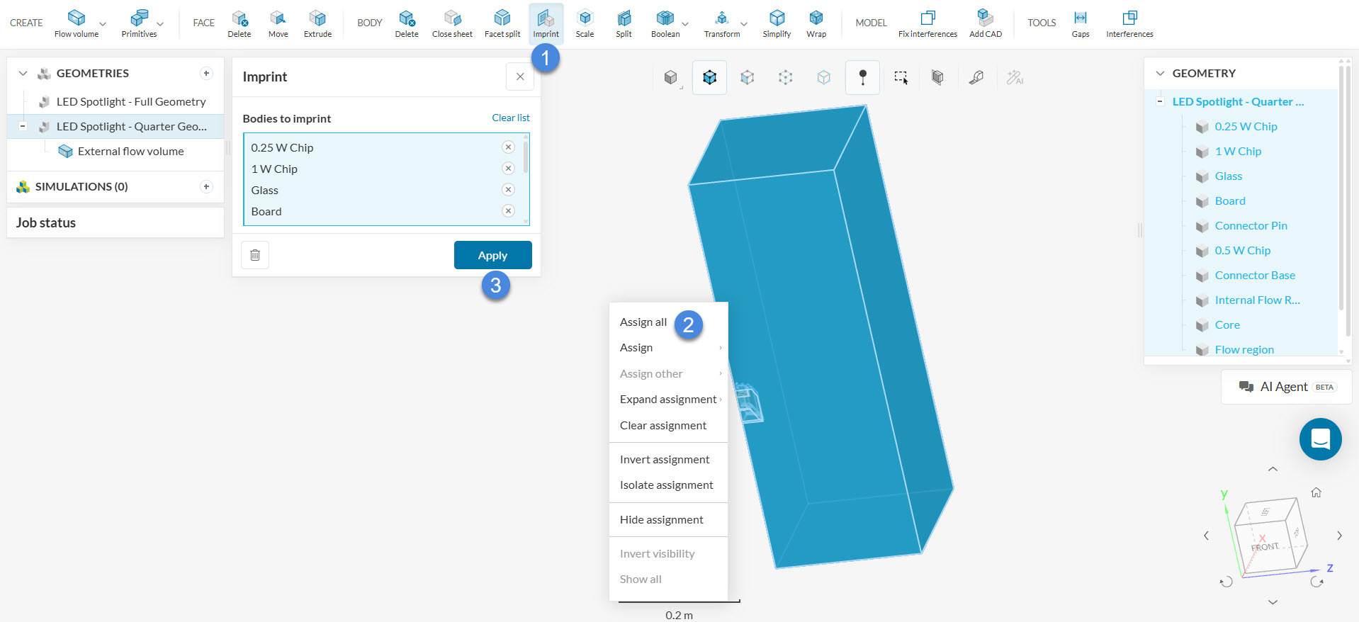
Once you finish running the imprint operation, all changes will be automatically saved to the selected geometry.
1.3. Create the Simulation
Once the geometry is ready, it will have the same name. In case you would like, you can always change the name of the new geometry to something more representative. After saving the name change, we are ready to ‘Create a Simulation’.
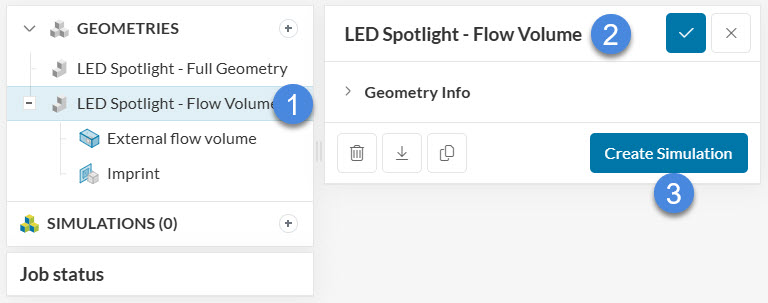
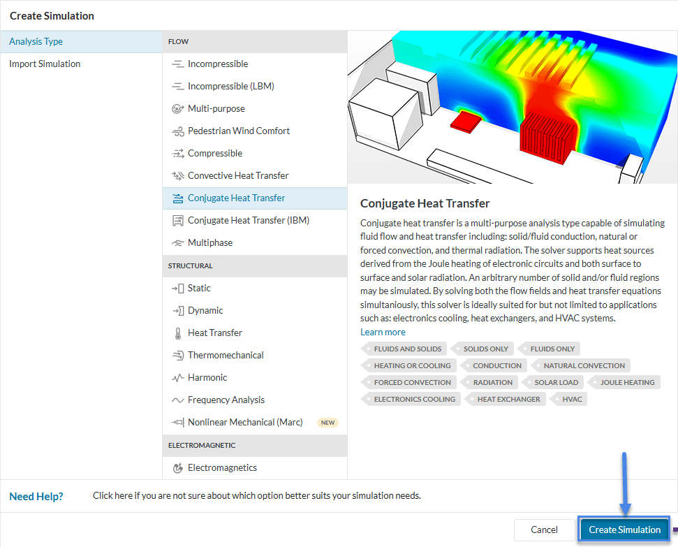
The analysis type choice widget opens up. From the options, pick ‘Conjugate Heat Transfer’ and ‘Create the Simulation’:
Did you know?
The analysis type you choose within the simulation library depends on what results you are interested in, and what given parameters you have.
- With a Conjugate Heat Transfer analysis type, it’s possible to simulate heat transfer between solids and also between the solid and fluid domains. This is the common choice for electronics cooling.
- If you are only interested in the heat transfer within solids, you can simplify the simulation process by performing a Heat Transfer analysis.
- Lastly, for simulating heat transfer only in the fluid domain, the appropriate analysis type is a Convective Heat Transfer.
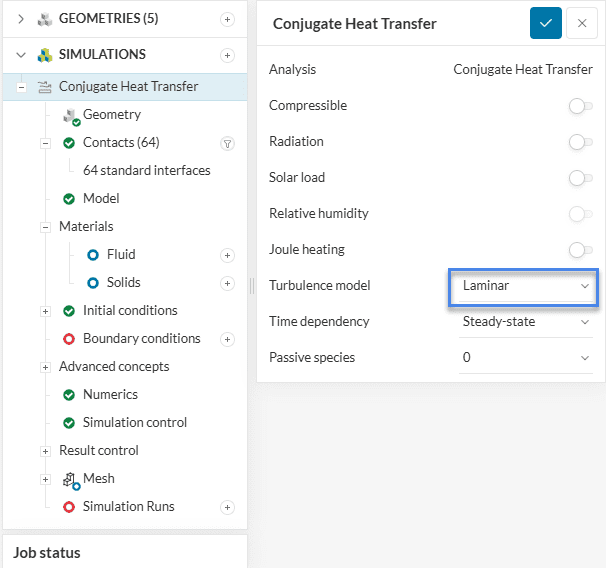
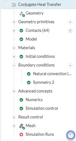
After creating a simulation, the simulation tree will be visible in the left-hand side panel. It’s necessary to set up all entries to be able to run the simulation. At this point, SimScale will also automatically detect all Contacts within the geometry. In our case, there are a total of 64 interfaces.
The global simulation settings are shown in Figure 11. Since it’s a natural convection simulation, the velocities in the domain are small, and a ‘Laminar’ turbulence model is appropriate.
Did you know?
In natural convection simulations, where the temperature gradients in the air domain are small, it’s common to use the Boussinesq approximation to account for buoyancy.
In Figure 11, one can use the Boussinesq approximation by keeping Compressible toggled off. For further information, please check this documentation page about buoyancy.
2. Simulation Setup
In the following sections, we will set up the physics of the simulation.
2.1. Model
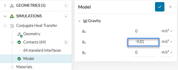
In the Model tab, it’s possible to define the direction and magnitude of gravity:
Please define gravity as ‘-9.81’ \(m/s^2\) in the y-direction.
2.2. Defining the Materials
In conjugate heat transfer simulations, it’s necessary to define both solid and fluid materials. Let’s first go through the fluid domain.
Important
Each volume in the domain needs to receive one material assignment.
Assigning more than one material to a volume or leaving parts without any assignments will result in an error.
2.2.1 Fluid Materials
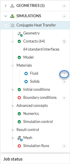
To add a fluid material, please click on the ‘+ button’ next to Fluid:
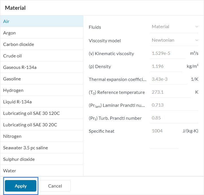
The fluid material library pops up. From the list, choose ‘Air‘ and hit ‘Apply’:
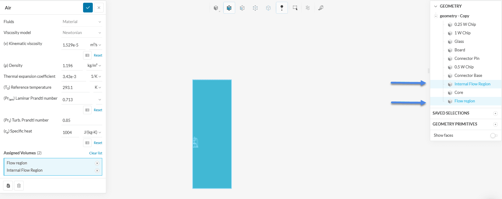
The geometry contains two air regions: one internal to the LED, and the external flow region. You can use the right-hand side panel to quickly select the volumes.
Did you know?
For this tutorial, we will use the default values for the air properties. It’s possible, however, to edit each one of the values from Figure 15 by clicking on them. Find more details about using custom materials in this article.
2.2.2 Solid Materials
Let’s now add the solid materials. First, click on the ‘+ button’ next to Solids, as in figure 12. This time, a library of solid materials appear.
From the list, please choose ‘PVC’, which is a common material for circuit boards:
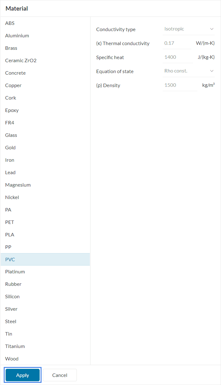
The materials library contains common properties for PVC. In this tutorial, PVC is used in a circuit board, so we will adjust the material properties to account for the circuits. Figure 17 shows the changes:
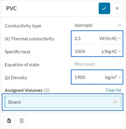
- Set \((\kappa)\) Thermal conductivity to ‘2.5’ \(\frac {W}{m.K}\).
- The new Specific heat is ‘1004’ \(\frac {J}{kg.K}\).
- Set \((\rho)\) Density to ‘1900’ \(\frac {kg}{m^3}\).
- Lastly, assign the Board volume.
All the remaining solid materials maintain the default settings. Find below a list of materials and the respective assignments.
- Aluminium: Core
- Brass: Connector Base
- Copper: Connector Pin
- Glass: Glass
- Silicon: 0.25 W Chip, 0.5 W Chip, and 1 W Chip
2.3. Initial Conditions
In CFD simulations, it’s a good practice to initialize the parameters close to the expected solution. With this approach, it’s possible to improve the convergence rate of a simulation, achieving the final result faster.
In this tutorial, we will change the initialization of temperature and velocity.
Did you know?
In SimScale, there are two ways to define the initialization of a parameter:
- Uniform initialization, which initializes a parameter in the entire domain with the same value
- Subdomain initialization, which initializes a parameter in specific volumes within the domain
For additional information on domain initialization, please visit this documentation page.
2.3.1 Temperature
The LED geometry contains three chips, which are dissipating heat. From a design perspective, it’s important to keep the chip temperatures under control, otherwise, the lifetime of the LED, along with the LED performance, becomes shorter.
Usual temperatures on the chips are around 100 \(°C\), thus, initializing the LED parts at 75 \(°C\) is a good initial guess. Figure 18 shows the initial steps for initialization with subdomains.
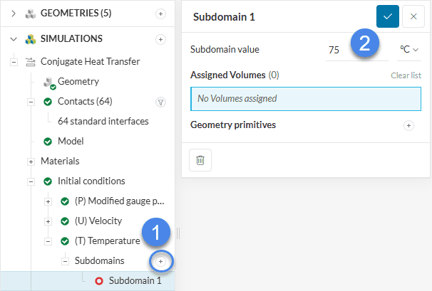
- Add a new subdomain by clicking on the ‘+ button’ next to Subdomains.
- Input the initialization value, in this case, ’75’ \(°C\).
We want to assign all the LED parts to this subdomain. The quickest way to do that is by using an Invert visible assignment function. Please proceed as below:
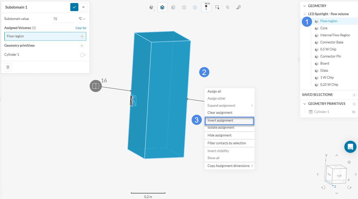
- Select the Flow region volume.
- By right-clicking in the viewer, a window with options appears.
- Click on Invert visible assignment. This way, the 9 volumes of interest are assigned.
2.3.2 Velocity
As a result of the high temperatures on the LED geometry, a natural convection plume develops. Therefore, we strongly recommend initializing the velocity field around the LED, which enhances the convergence rate of the simulation.
In this tutorial, we will initialize the velocity field using a cylinder geometry primitive, which is a good option for the shape of the LED geometry. Figure 21 shows the initial steps:
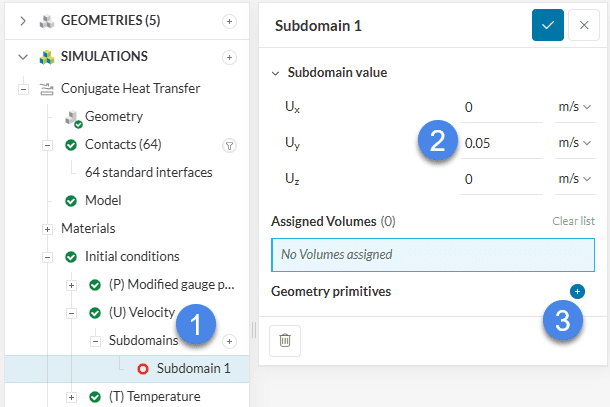
- Add a new subdomain by clicking on the ‘+ button’ next to Subdomains.
- Using the orientation cube as a reference, initialize the velocity in the y-direction with ‘0.05’ \(m/s\).
- Click on the ‘+ button’ next to Geometry primitives and select a ‘Cylinder’.
Now, a window opens up, where the user can define the cylinder orientation and dimensions. Using a cylinder slightly wider than the LED geometry yields good results. Therefore, please input the values from Figure 22:
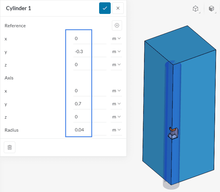
After saving the cylinder primitive, it is automatically assigned to the velocity subdomain.
Important
The optimal value for the velocity initialization may vary from case to case. For natural convection applications, initializing velocity with velocities between 0.05 and 0.2 m/s provides a very good convergence in most cases.
2.4. Boundary Conditions
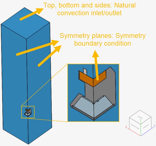
For boundary condition definition, we will use Figure 23 as reference:
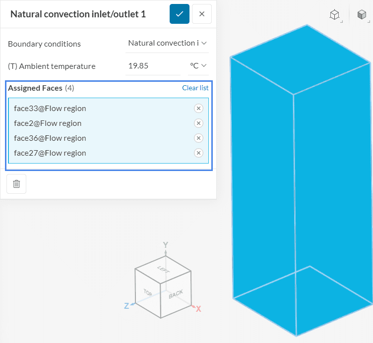
2.4.1 Natural Convection Inlet/Outlet
The natural convection inlet/outlet boundary condition is exclusive to SimScale. This boundary condition allows fluid to go in and out of the domain, therefore it’s a good option when it’s not clear what the flow behavior will be. For more details on the mathematical implementation, see this dedicated documentation page.
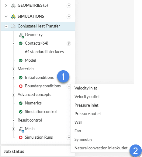
To create a new boundary condition, click on the ‘+ button’ next to Boundary conditions, and select the desired type from the drop-down menu.
Using figure 23 as a reference, the top, bottom, and both side faces will receive a natural convection inlet/outlet boundary condition.
2.4.2 Symmetry
Please create a second boundary condition, as in figure 24. This time, however, select a Symmetry condition:
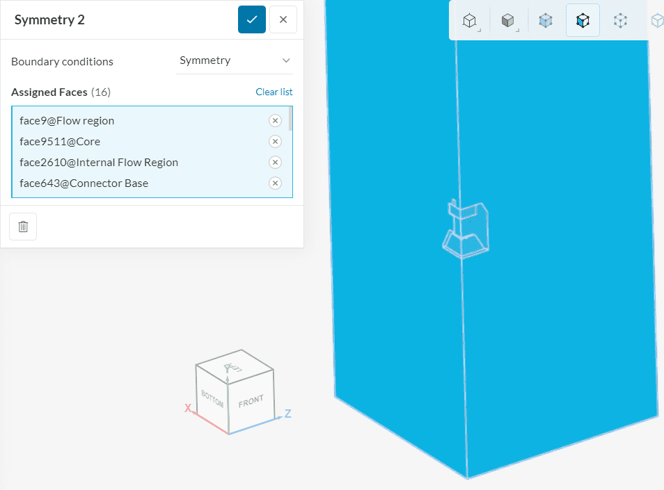
Note
Please note that all 16 faces in the symmetry plane receive a symmetry boundary condition. This includes all faces shown in Figure 27.
2.5. Advanced Concepts
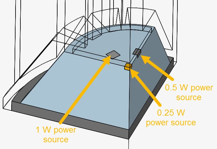
Additionally, the geometry contains three chips, which will be defined as power sources. Figure 28 contains further details:
In SimScale, there are two types of Power sources:
- Absolute power source: the user defines the heat flux in \(W\) or \(\frac {btu}{s}\)
- Specific power source: the definition of the flux is in \(W/m^3\) or \(\frac {btu}{s.in^3}\)
Hence, the Absolute power source works best in our case, as we already know the exact heat flux in each chip.
Please proceed to set up the first power source, as in Figure 29:
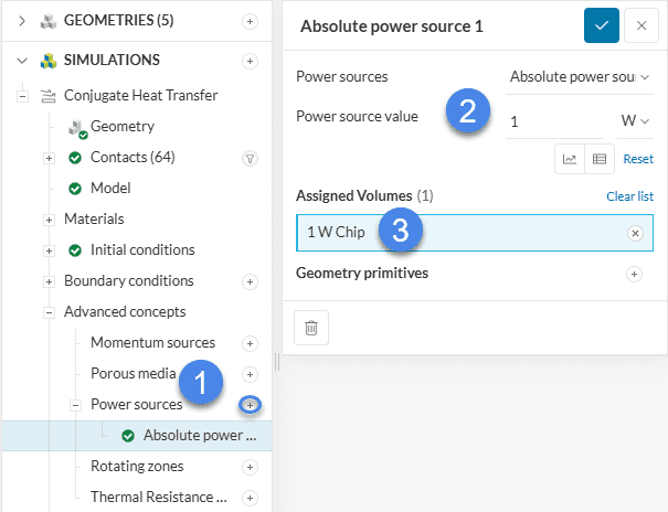
- Create a new power source by clicking on the ‘+ button’ next to Power sources.
- Select an ‘Absolute power source’ and set the heat flux to 1 watt.
- Assign the 1 W Chip volume to this power source, which can be done using the right-hand side geometry panel in the Workbench.
Please create two new power sources, for the 0.5 W Chip and the 0.25 W Chip volumes. Follow the same steps outlined above, remembering to adjust the Heat flux accordingly.
2.6. Numerics & Simulation Control
The default settings in the Numerics tab work well for most simulations. In this tutorial, no changes are required.
In the Simulation control tab, it’s possible to define a series of parameters that control the simulation process, including the number of iterations to perform, and the maximum runtime for the simulation run. Figure 30 highlights the changes in the simulation control tab:
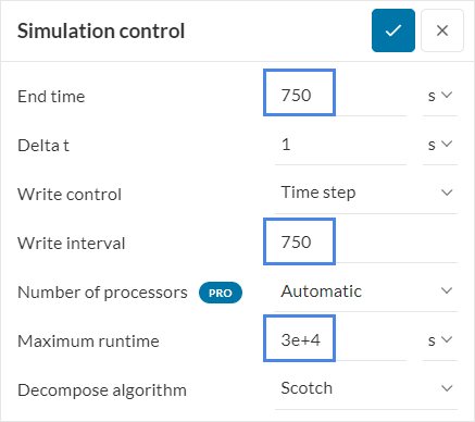
- Define an End time of ‘750’ iterations and a Write interval of ‘750’ iterations. With these settings, only the result set from the last iteration will be written, which is a common practice for steady-state simulations.
- Change the Maximum runtime of the simulation to ‘30000’ seconds.
Did you know?
In a steady-state simulation, the End time and Delta t parameters control the number of iterations to be performed.
For more notes on the simulation control settings, please visit the following page: Simulation Control for Fluid Analysis
2.7. Results Control
Setting up result controls is a crucial step in a simulation. Since they help us to assess convergence, it’s important to set meaningful result controls for our parameters of interest.
For a LED simulation, some parameters of interest are, for example, the temperature on the chips. Therefore, we will set Area average result controls on them. To do that, please proceed as in Figure 31:
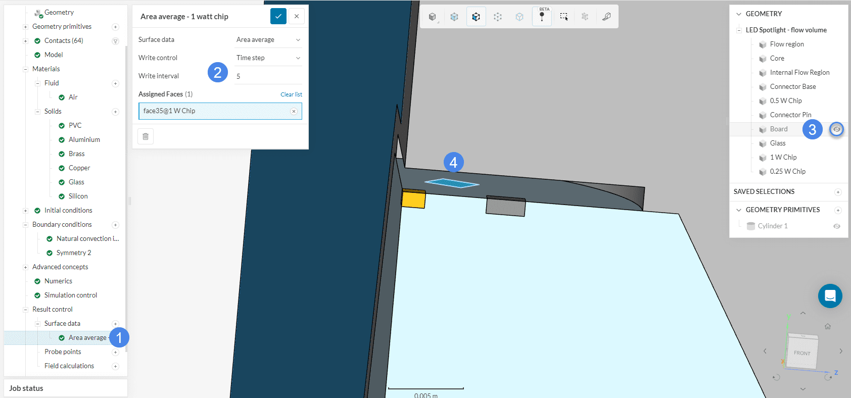
- Create a new Area average control by clicking on the ‘+ button’ next to Surface data.
- Define a Write interval of ‘5’ iterations. This way, the algorithm will plot the area averages every 5 iterations, which is good enough for a steady-state simulation.
- To make the face selection easier, please hide the Board volume, by clicking on the ‘eye icon’ next to it.
- For the first result control, please select the top face of the 1-watt chip.
Afterward, following the same procedure, please create two additional area average controls, for the top faces of the 0.5 W Chip and the 0.25 W Chip.
3. Mesh
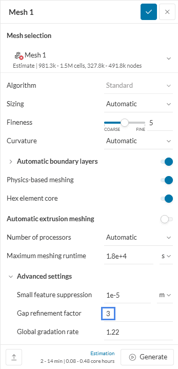
For the meshing operation, we recommend using the standard algorithm, which is a good choice in general, as it is quite automated and delivers good results for most geometries.
After clicking on Mesh in the simulation tree, a setup window opens. The main default settings are good for an initial study. Under Advanced settings, please set the Gap refinement factor to ‘3’.
Did you know?
In CHT simulations, oftentimes the solid parts will have thin sections. It’s important to add at least 2 or 3 cells to correctly resolve the temperature gradients within these small parts.
By defining the Gap refinement factor to 3, the meshing algorithm will ensure at least 3 elements capturing the small sections.
With these mesh settings, we already have a good mesh that allows us to run a successful simulation.
In the box below, we will show optional steps to configure a volume custom sizing for the mesh, which allows us to capture the convection plume more accurately. If you would like to proceed without volume custom sizing, please skip to section 4.
(Optional) Volume custom sizing for the convection plume
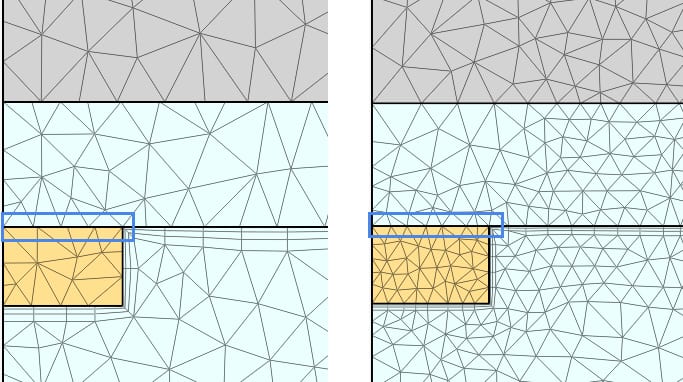
In natural convection simulations, a convection plume develops above the hot parts. To capture the plume more accurately, we can use finer mesh cells around that region.
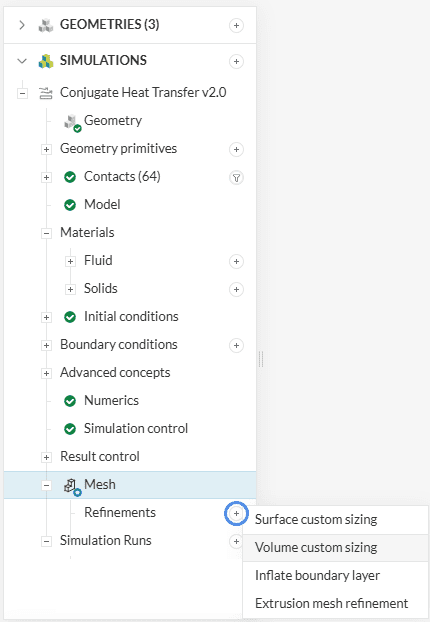
With the standard mesher, a volume custom sizing is appropriate to capture the developing plume. Therefore, please click on the ‘+ button’ next to Refinements:
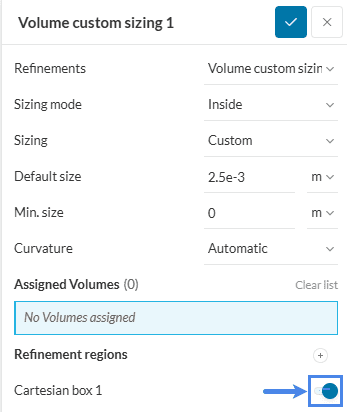
In the configuration window that opens, you can modify the Sizing from Automatic to Custom and edit the Default size for the cells inside the volume region. In Figure 36, you will find the necessary steps:
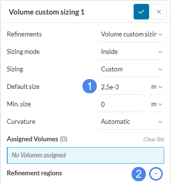
1. Define a Default Size of ‘0.0025’ meters
2. Click on the ‘+ button’ next to Volume custom sizing and choose a ‘Cartesian box’
Next, it’s necessary to define the dimensions of the cartesian box. Keeping the convection plume in mind, please input the following dimensions:
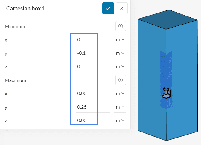
- Minimum (x) value: 0 \(m\)
- Minimum (y) value: -0.1 \(m\)
- Minimum (z) value: 0 \(m\)
- Maximum (x) value: 0.05 \(m\)
- Maximum (y) value: 0.25 \(m\)
- Maximum (z) value: 0.05 \(m\)
As a final step, return to the Volume custom sizing previously created, and toggle on the cartesian box assignment.
This concludes the configuration of the Volume custom sizing.
Did you know?
The CHTv2.0 solver uses a special kind of meshes, named conformal meshes. In a conformal mesh, the faces of the cells at the interface between two parts will match perfectly, which allows for a more robust setup and faster convergence.
For this reason, meshes created for other analysis types can’t be used in a CHTv2.0 simulation.
4. Start the Simulation
To start a new simulation, please click on the ‘+ button’ next to Simulation Runs.
This way, the mesh will be generated, and afterward, the simulation run will start automatically. While the simulation results are being calculated, you can already have a look at the intermediate results in the post-processor. They are being updated in real-time! You will also find a link to the finished project at the end of the tutorial.
The simulation run takes from 1 to 2 hours to finish. At this point, you can access the post-processing environment by clicking on ‘Solution Fields’ or ‘Post-process results’:
5. Post-Processing
5.1 Result Controls
Before heading over to the post-processing environment, let’s inspect the data obtained with the result controls. The average chip temperatures are available under the ‘Area averages’ tab:
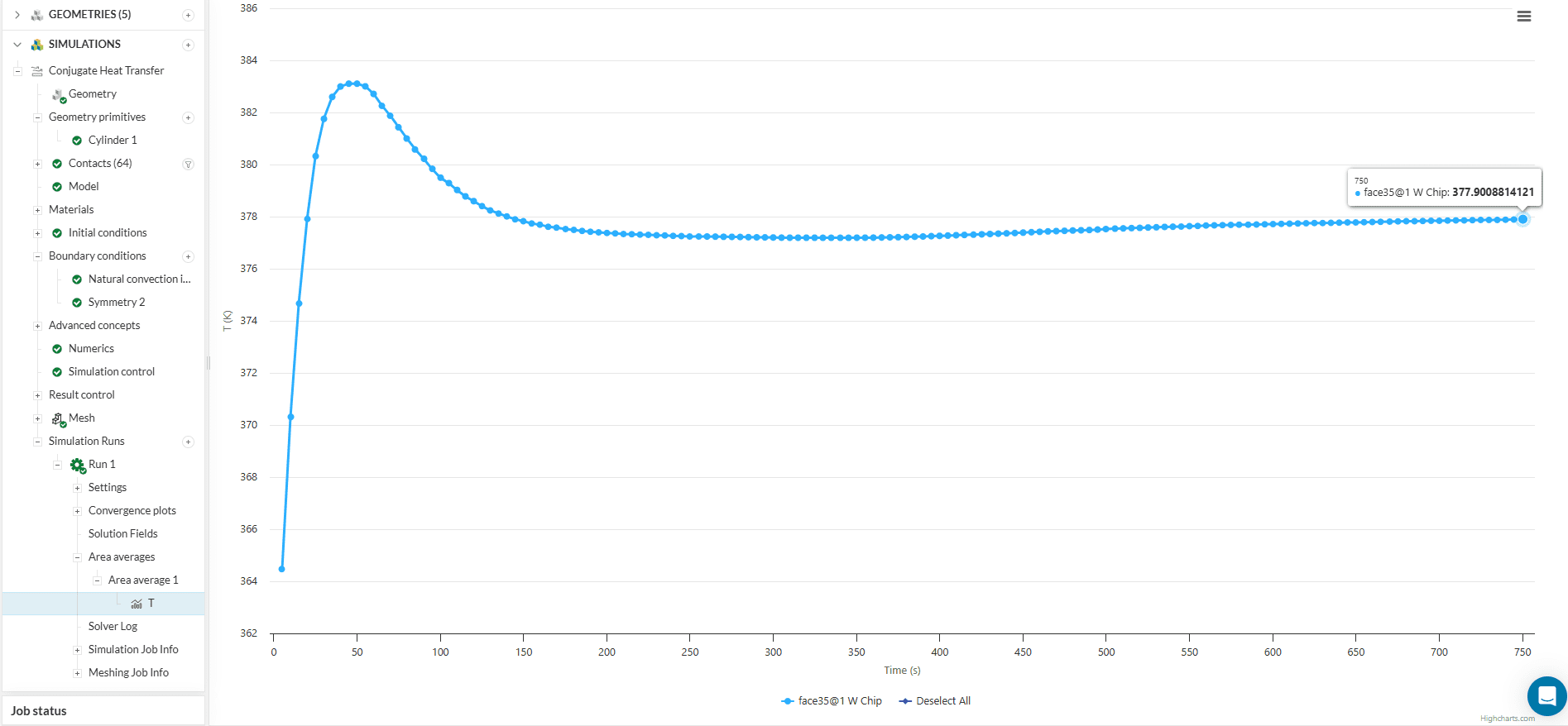
The plot shows how the chip temperature is evolving as the algorithm performs iterations. In a converged simulation, the temperatures will stabilize and no longer change between iterations. As a result of the strongly coupled formulation from the CHT algorithm, the temperature converges quickly, in just over 300 iterations.
For more notes on assessing convergence in CFD simulations, please refer to this article.
Did you know?
With SimScale, it’s possible to run multiple simulations in parallel for different LED designs. The aim is to obtain an optimized geometry, with lower temperatures on the chips.
This way, you can evaluate various geometries faster, speeding up the design process.
5.2 Temperature Contours
For electronics cooling applications, it is useful to visually evaluate the temperature on and around the chips. After accessing the post-processor by clicking on ‘Solution Fields‘, please proceed as below:
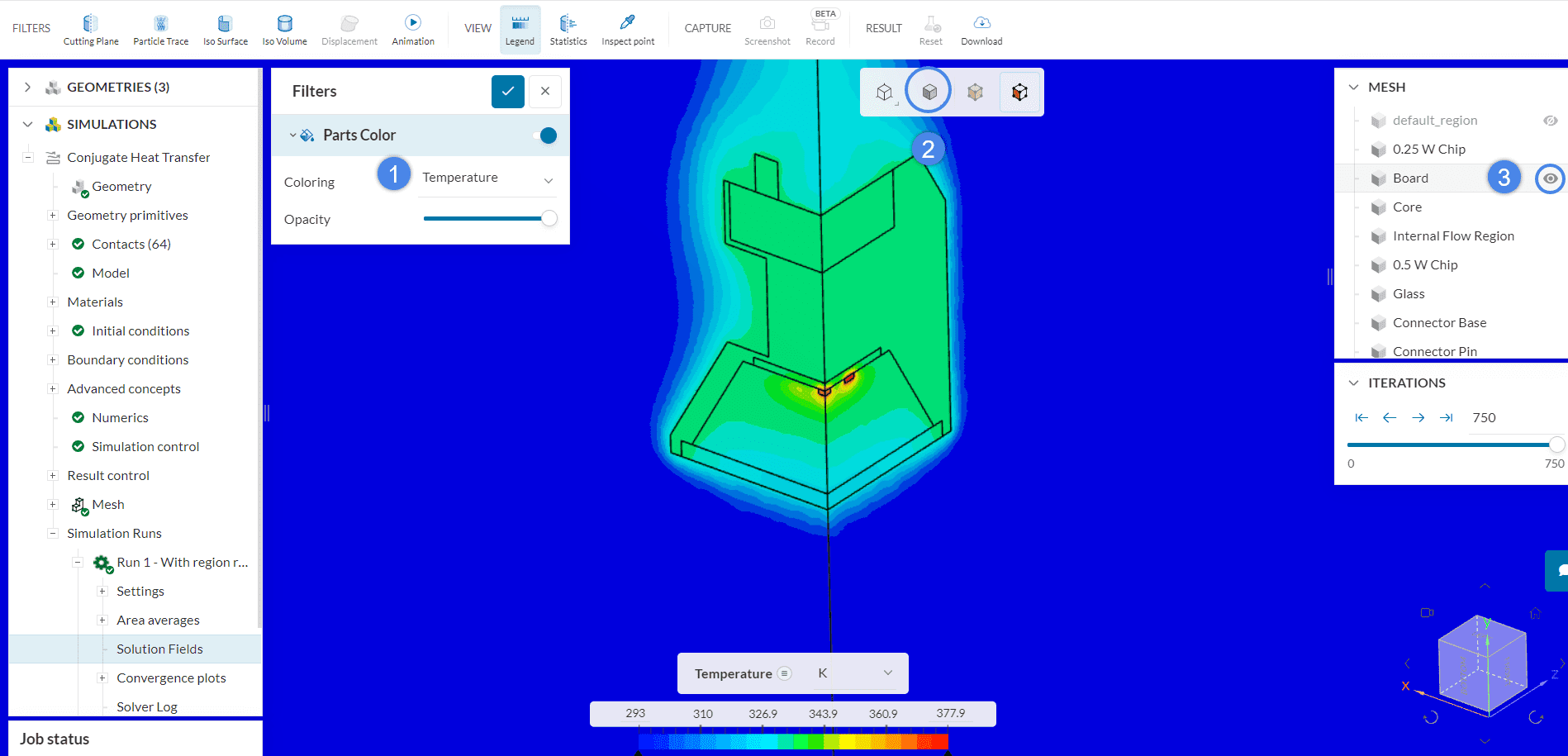
- Set the Coloring under Parts Color to ‘Temperature’. Now the temperature is shown in the viewer.
- To make the visualization better, we can also adjust the render mode. Both Surfaces with wireframe and Translucent surfaces with wireframe work nicely for this purpose.
- On the right-hand side panel, click on the ‘eye icon’ next to Board. This way, we will be able to see the temperatures on the chips clearly.
Now that we have a free view of the chips, we can also use the Inspect point feature to dynamically inspect points of interest. The image below shows the steps:
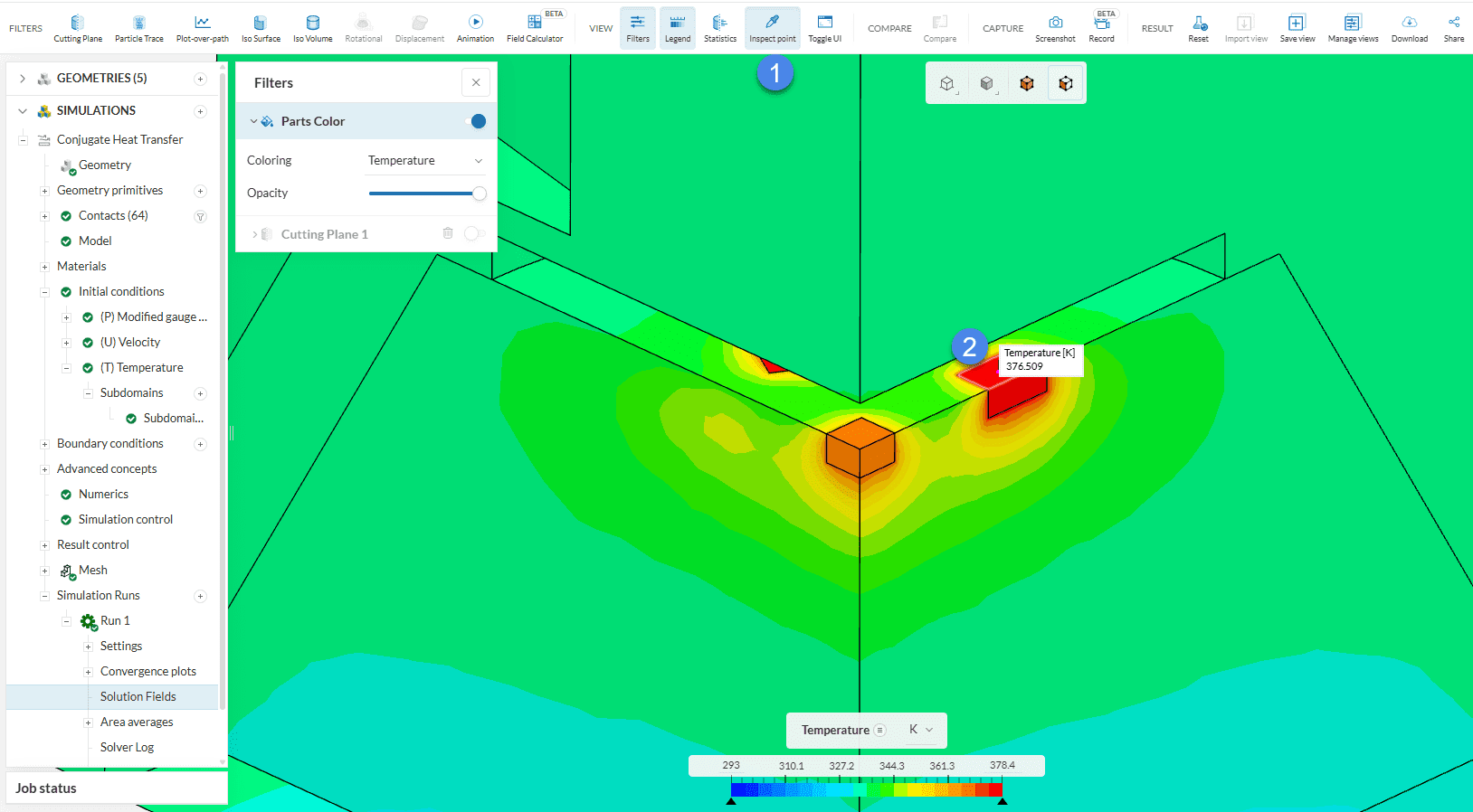
- Select the ‘Inspect point’ feature on the top bar
- After making sure that the Board volume is hidden, you will be able to inspect the temperature directly on the chips. Adjust the camera angle and hide other volumes if necessary
5.3 Particle Traces and Animations
After accessing the post-processor by clicking on ‘Solution Fields‘, you can use several post-processing filters to further analyze the results.
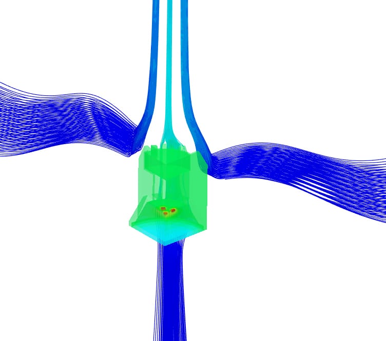
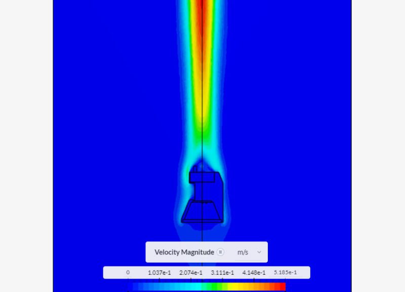
For example, the Particle Trace filter tracks the particles as they move through the domain. This filter is very useful to capture the convection plume that forms due to the convection effects. Please proceed as below:
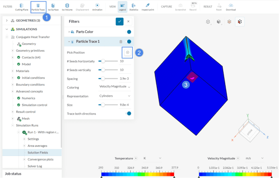
- Create a new filter by clicking on the ‘Particle Trace’ button on the top ribbon
- Make sure that the Pick Position button is on. This way, you can define the seeds for the traces
- By selecting a face under the LED, you will be able to see the convection plume forming
It is possible to create even more particle trace filters, so we can see how the air moves from multiple different positions. For example, some air is drawn from the sides of our flow region, due to the convection plume that is generated. Create a second particle trace filter, this time, selecting one of the side walls:
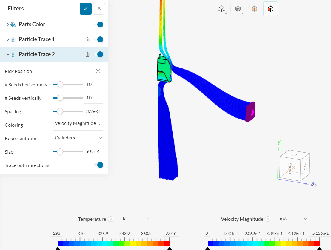
Particle trace filters are even more powerful when animated. Now that we have a couple of particle traces, let’s create an ‘Animation’ filter for them. Remember to change the Animation type to ‘Particle Trace’ before starting the animation:
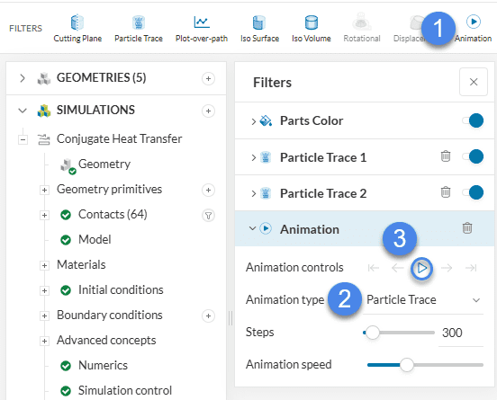
After pressing the play button (step 3 in the image above), we can see how the particles travel through the domain in the animation:
With the current configuration, we are getting temperatures around 375 \(K\) on our chips. With the insights obtained from this initial simulation, we have more information to optimize the following iterations and achieve lower temperatures.
Have a look at our post-processing guide to learn how to use other filters from the post-processor for this simulation.
Note
If you have questions or suggestions, please reach out either via the forum or contact us directly.
Last updated: April 6th, 2026
Did this article solve your issue?
How can we do better?
We appreciate and value your feedback.


