Advanced Tutorial: Crash Test of FSAE Impact Attenuator
This article provides a step-by-step tutorial for a dynamic simulation of an FSAE Impact Attenuator.
Overview
This tutorial teaches how to:
- Set up and run a dynamic simulation.
- Assign boundary conditions, material, and other properties to the simulation.
- Mesh with SimScale’s Standard meshing algorithm.
You are following the typical SimScale workflow:
- Prepare the CAD model for the simulation.
- Set up the simulation.
- Create the mesh.
- Run the simulation and analyze the results.
Attention!
This tutorial performs simulation with the Dynamic analysis type which is only accessible to users with a Professional plan and those who are already on the Community plan. New Community users or those recently downgraded to the Community plan will no longer be able to perform this tutorial. See our pricing page to request additional features.
1. Prepare the CAD Model and Select the Analysis Type
To start with the tutorial, please click on the button below. This will create a copy of the tutorial project in your Workbench.
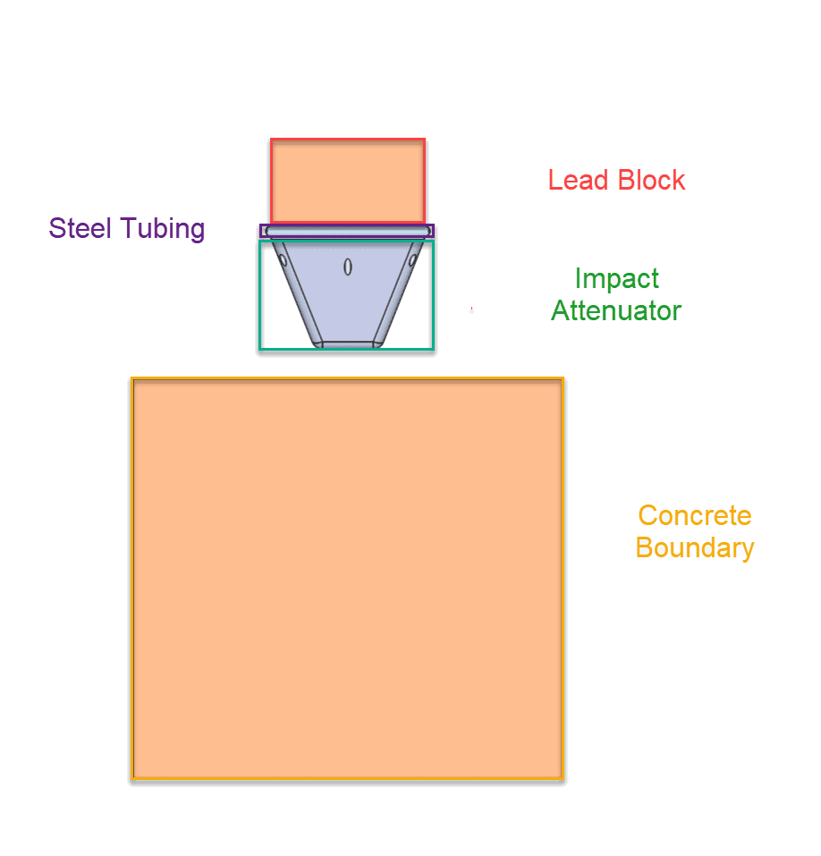
The following picture demonstrates what should be visible after importing the tutorial project.
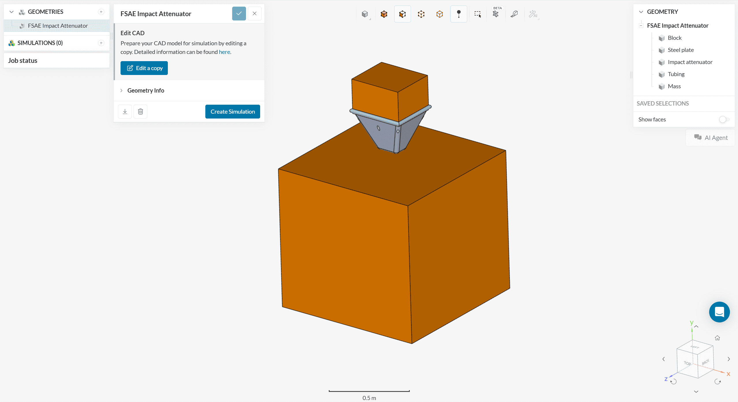
This is the standard Formula SAE Impact Attenuator (IA). The job of the impact attenuator is to reduce the maximum acceleration of the driver during an impact to ensure driver safety. The IA is attached to a steel tube frame, with a lead block that represents the mass of a moving car. Finally, the concrete block is a rigid structure that is the worst-case scenario for an impact.
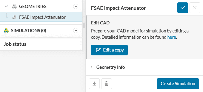
1.1. Create the Simulation
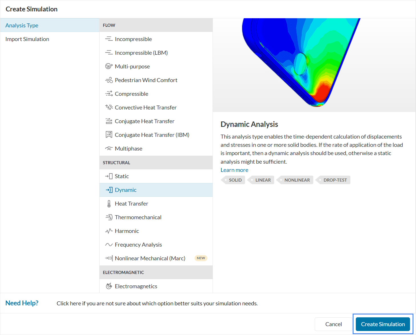
Start by clicking on the new geometry, and then on the ‘Create Simulation‘ button.
Hitting the Create Simulation button leads to several CFD and FEA options. Select ‘Dynamic‘ as the type of analysis.
2. Set Up the Simulation
2.1. Contacts
SimScale will automatically set any faces that perfectly touch within the geometry as Contacts, but sometimes assignments are needed for faces that SimScale won’t automatically pick up. For this tutorial, we will add more faces to the Bonded 2 contact and, later on, create a third bonded contact.
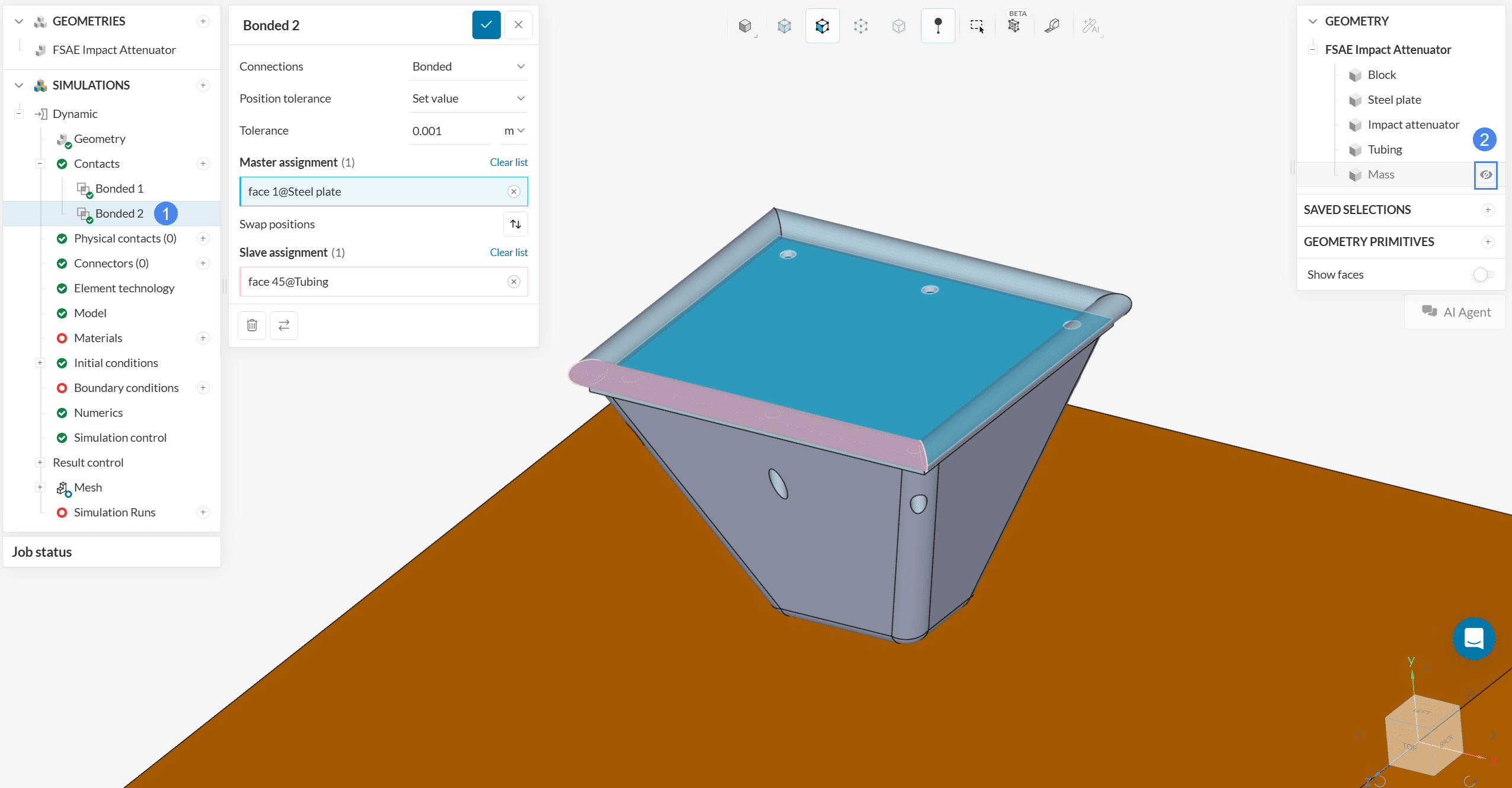
First, select the Bonded 2 contact and hide the Mass volume by clicking on the eye icon to allow the visualization of contact faces:
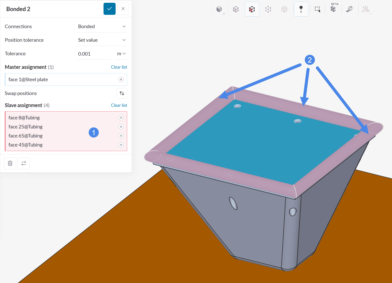
The bonded 2 contact is missing 3 slave assignments. As such, click on the Slave assignment box to activate it, and then click on the 3 missing faces, as shown below:
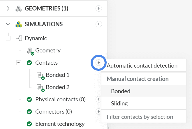
Next, a third bonded contact will be added. Please click the plus next to Contacts in the simulation tree and select ‘Bonded‘ under Manual contact creation.
This time, the tubing volume faces will be bonded to a face of the Mass volume:
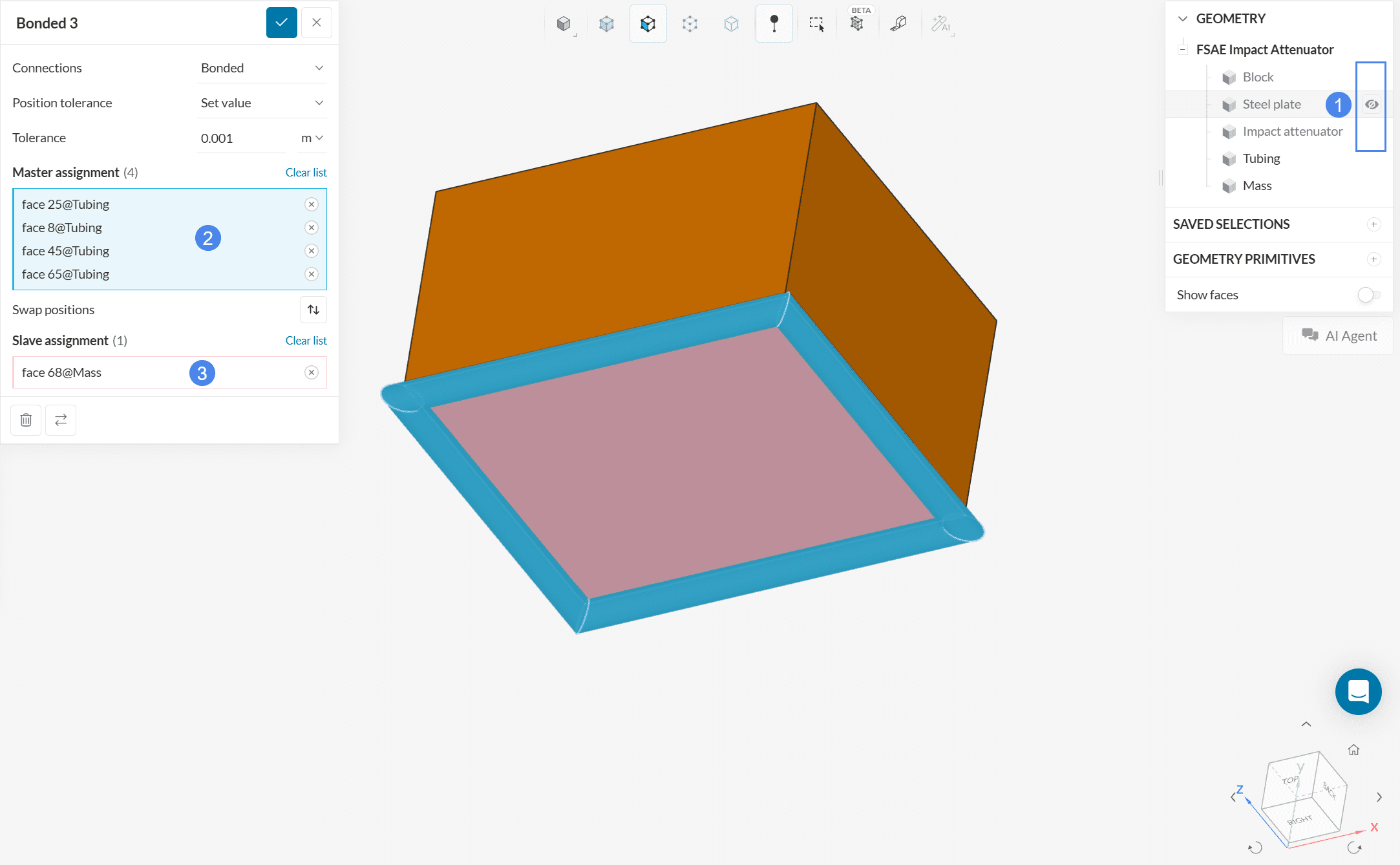
To make the face selection easier, hide the Block, Steel plate, and Impact attenuator volumes. Then select the 4 outer faces of the Tubing volume as the Master assignment and the bottom face of the Mass volume as the slave assignment.
It is important to be careful when assigning slave and master assignments. SimScale will not allow you to have multiple slave assignments on the same face. As shown above, the tubing faces were the slave assignment in Bonded 2, but the master assignment in Bonded 3.
After creating the bonded contacts, you need to set a Physical contact between the front faces of the impact attenuator and the impact block. This physical contact will allow the set of faces to interact with each other when the impact occurs.
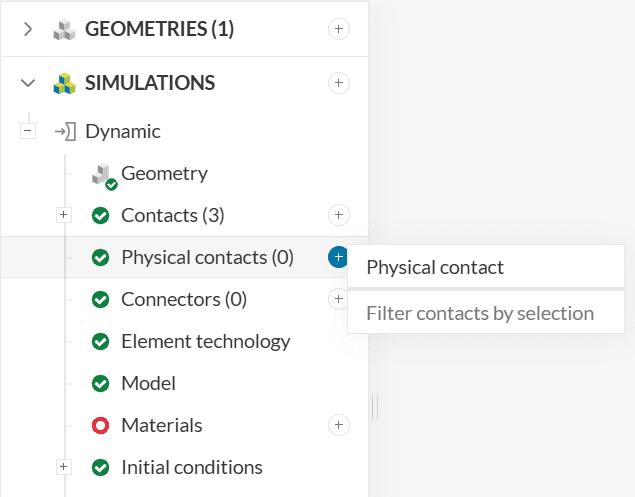
In this definition, the top face of the concrete Block will be the Master assignment, whereas the bottom faces of the Impact attenuator will be the slave assignments.
A total of 17 faces of the impact attenuator volume will be assigned as slave faces. We can use the tangent faces expand assignment functionality to quickly pick all of them.
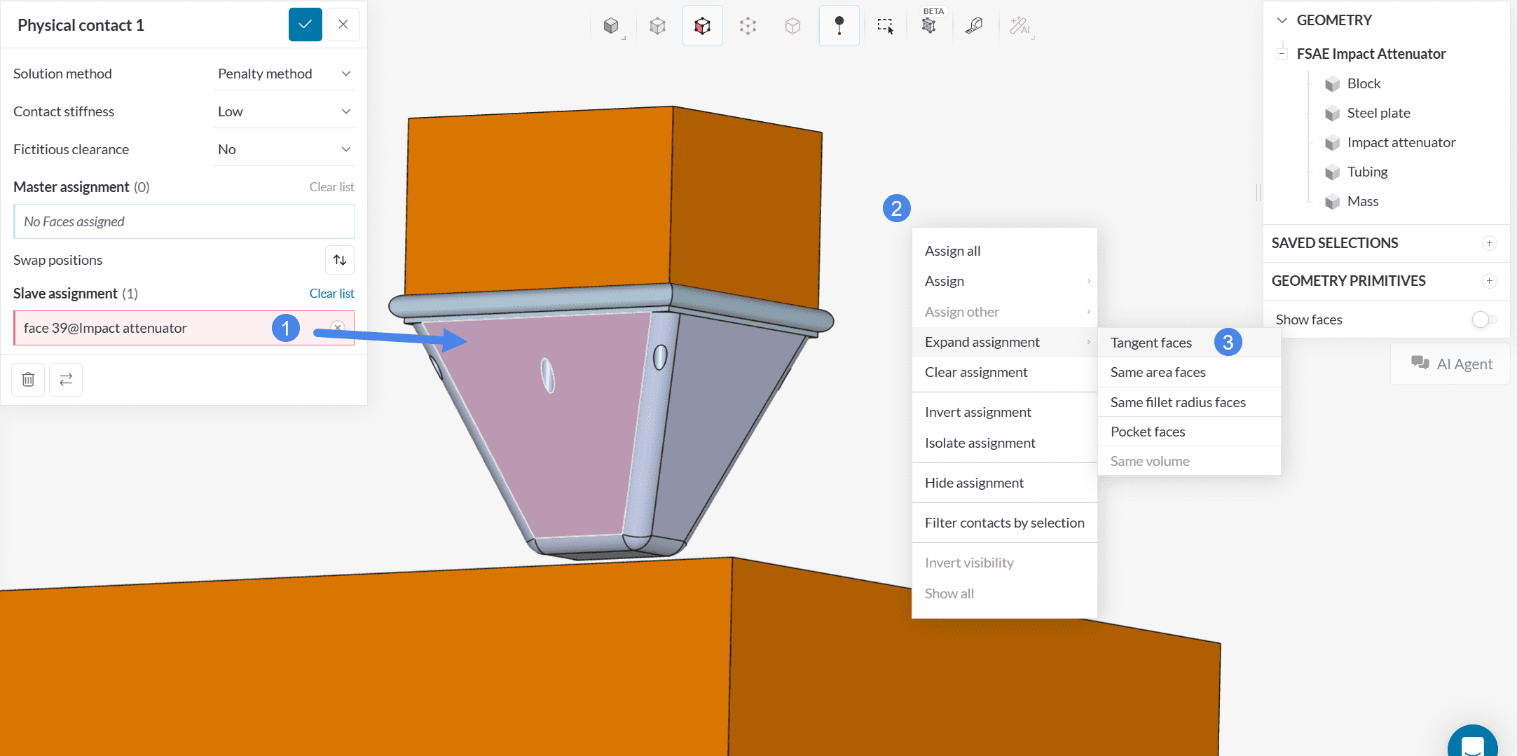
- Enable the Slave assignment box and select one of the impact attenuator faces
- Right-click on the viewer
- Navigate to Expand assignment and select Tangent faces. This will assign the remaining 16 faces as slave assignments, for a total of 17 faces.
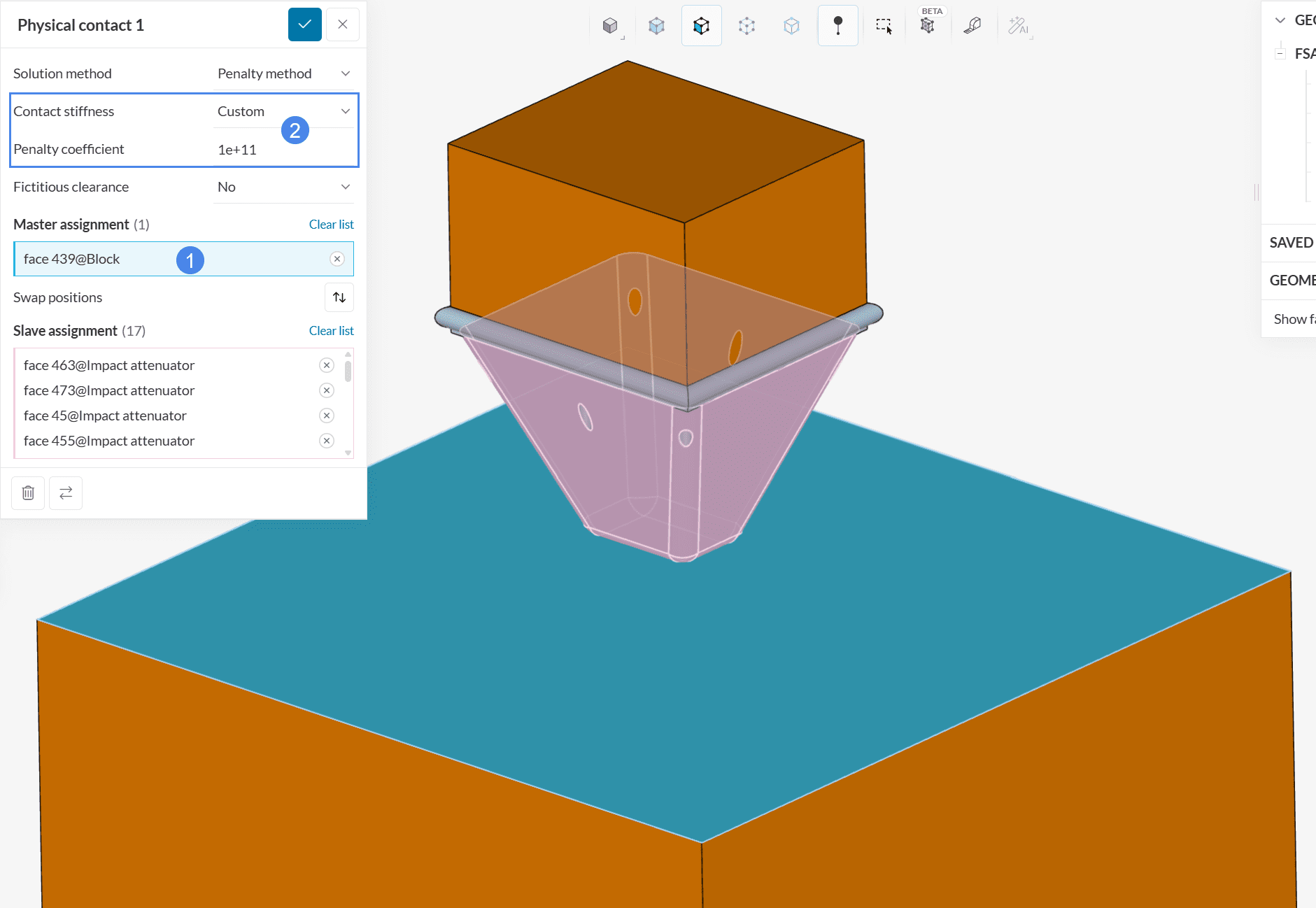
To finalize the physical contact setup, select the top face of the Block volume as a master assignment, and adjust the Contact stiffness to ‘Custom’ with a Penalty coefficient of ‘1e+11’.
2.2. Materials
The SimScale platform comes with many default materials. To add new materials, click on the ‘+’ icon next to the Materials in the simulation tree and select ‘Steel’ from the list.
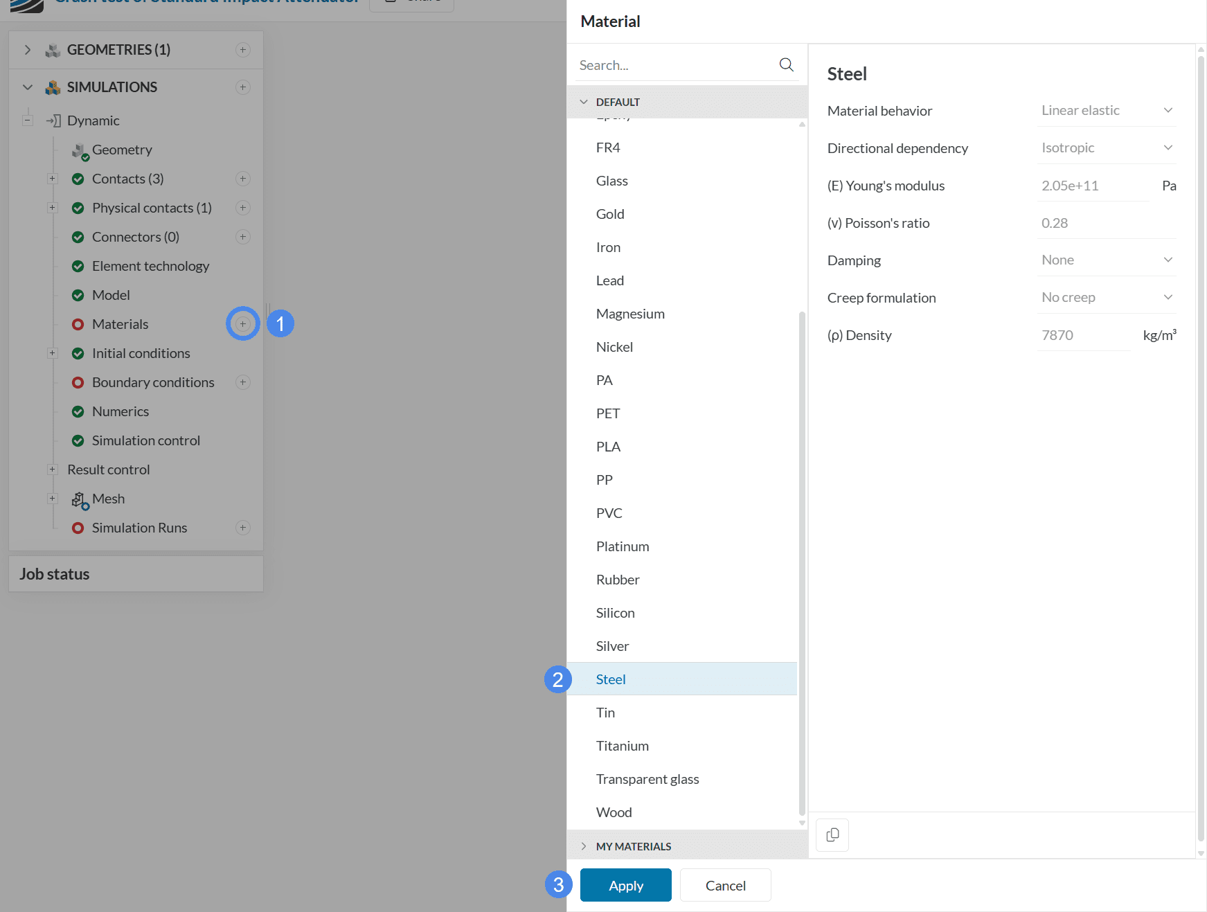
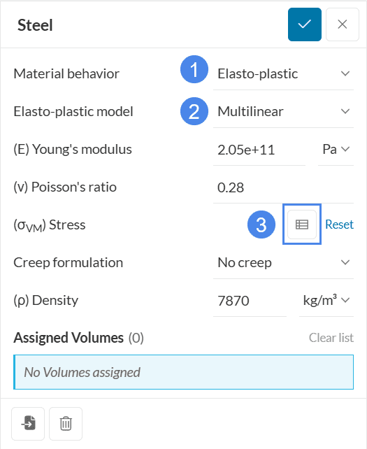
By default, the material behavior for steel is Linear elastic. For this simulation, please adjust the material behavior setting to ‘Elasto-plastic’. For this tutorial we want to define a full stress-strain curve, so please also switch the Elasto-plastic model to ‘Multilinear’. Then, you will be prompted to define the true stress-strain curve of the material by clicking on the table definition icon.
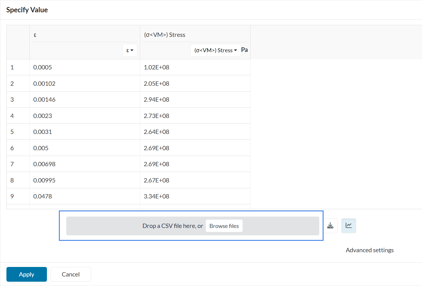
The stress-strain curve definition for steel can be found in the first sheet from this spreadsheet (named Steel – Tubing & Steel plate). Therefore, make sure to download the first sheet as a .csv file, and upload it to SimScale using the import box shown below.
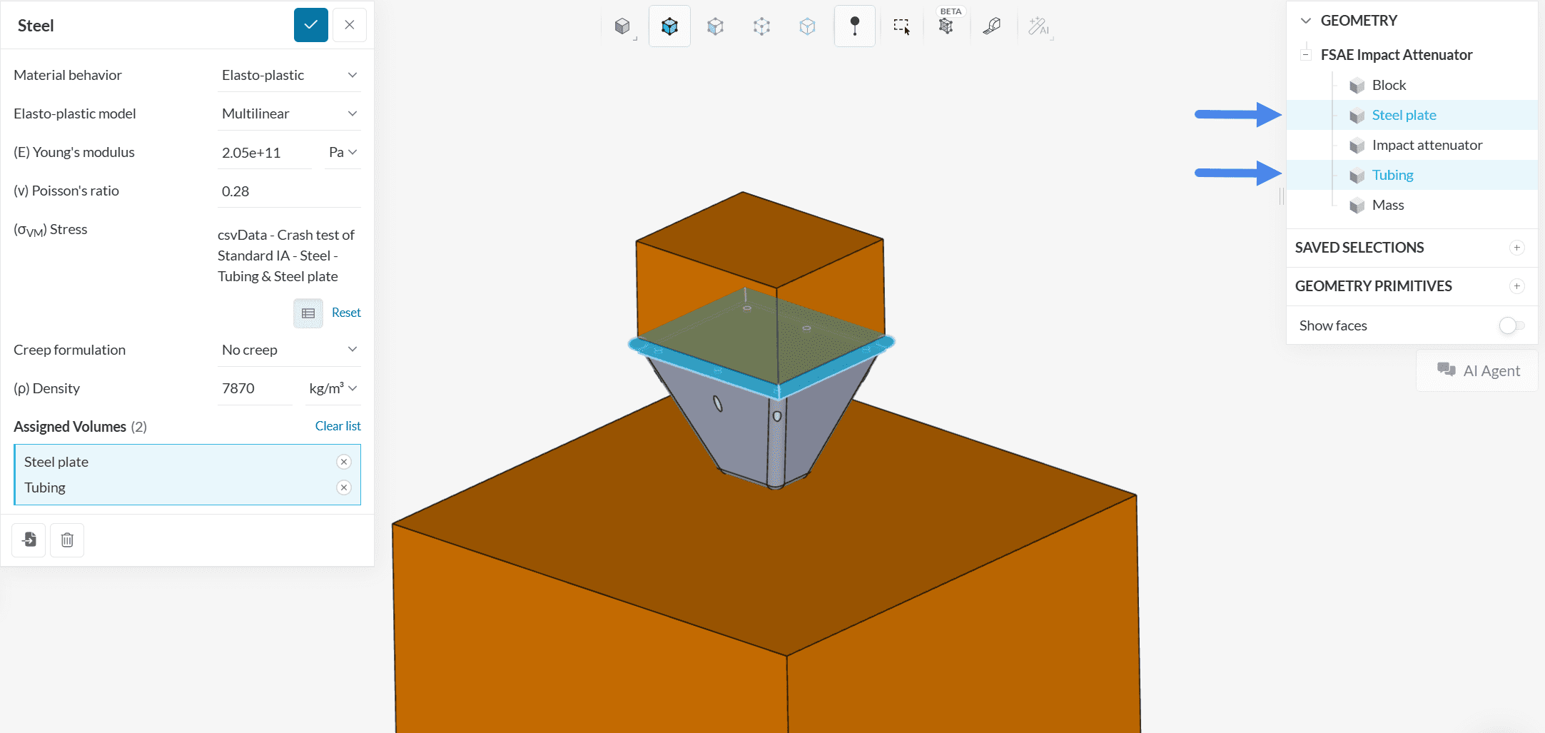
Finally, please assign this material to the ‘Tubing‘ and ‘Steel plate‘ by selecting them from the geometry tree at the right of the Workbench.
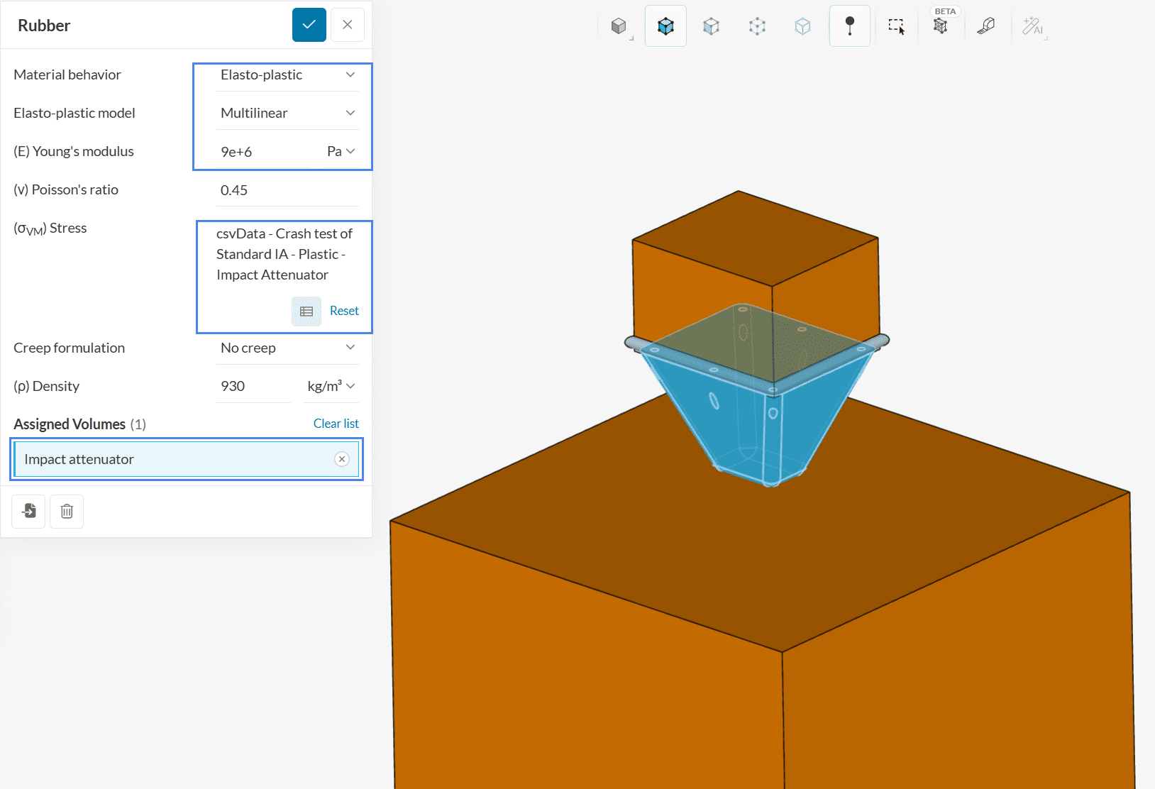
Create a new material, this time selecting ‘Rubber‘ from the Material list—this one will be used for the Impact Attenuator volume. Some changes will be performed on the default rubber settings:
- The new material behavior will be ‘Elasto-plastic’ with a ‘Multilinear’ Elasto-plastic model
- The Young’s modulus will be changed to ‘9e+6’ \(Pa\) due to the stress-strain data that will be defined (see more notes on Young’s modulus calculation on this documentation page).
- Find the stress-strain curve for the rubber material in the second sheet from this spreadsheet (named Plastic – Impact Attenuator). Again, downloading the data as a CSV file and uploading it to SimScale is the best way to proceed.
- Finally, assign the rubber material to the ‘Impact attenuator’.
Changing the material behavior to plastic allows the material to hold its deformation once a force is no longer applied. With the elastic behavior, the material will return to its original shape. The elastic behavior is suitable for small deformation simulations, but for larger deformations the plastic material behavior is essential.
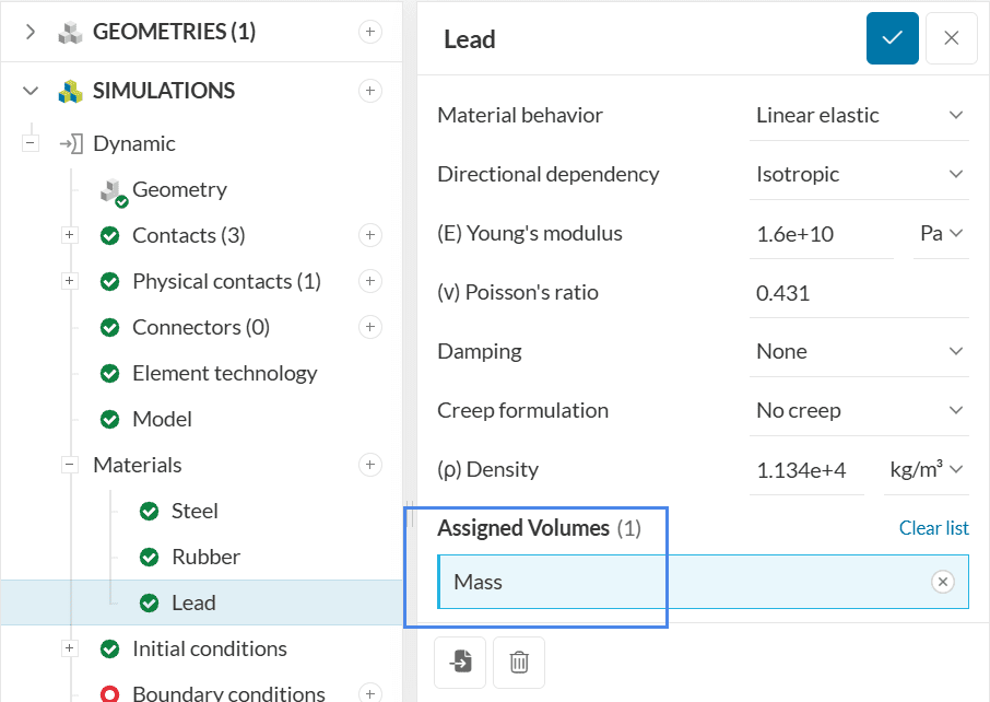
The next material from the list will be ‘Lead‘. Please assign it to the ‘Mass’ volume.
Repeat the same process, now with ‘Concrete‘ as the material, assigning it to the ‘Block’ volume with default settings.
2.3. Initial Conditions
For time-dependent simulations such as dynamic analyses, the initial conditions are very important, as they define the initial state of the system. In this tutorial, all volumes except for the concrete block will receive a velocity initialization:
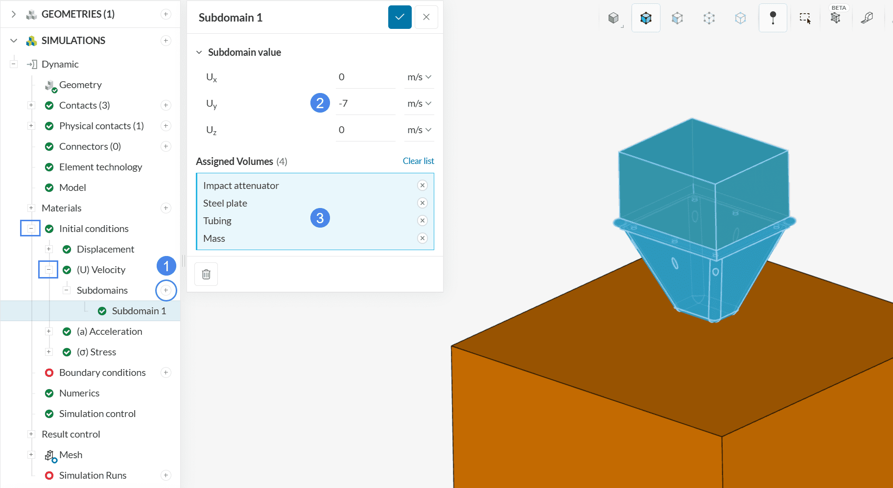
- Click on the ‘+’ icon next to the Subdomains, under (U) Velocity.
- Apply a velocity of ‘-7’ \(m/s\) in the Y direction.
- Assign this velocity initialization to the ‘Steel plate, Impact attenuator, Tubing, and Mass’ volumes.
2.4. Boundary Conditions
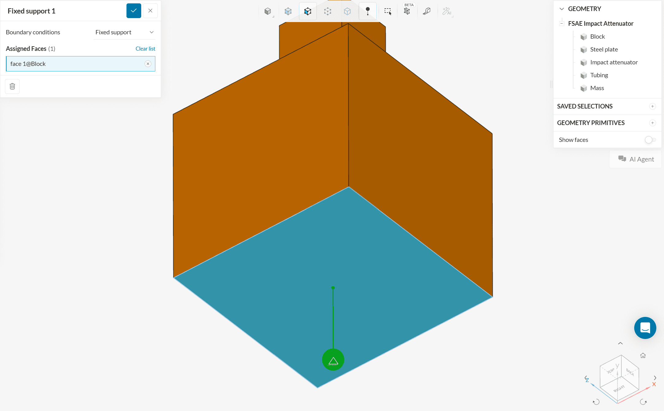
Up next, you can define constraints and loads via boundary conditions. In this tutorial, the base of the concrete block will be fully constrained with a Fixed support boundary condition:
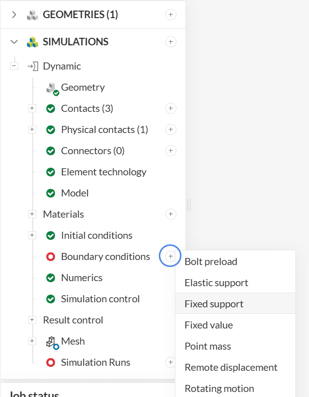
Rotate your model and click on the face on the bottom of the concrete block to fix it. This configuration will ensure that the base of the block doesn’t move during the collision.
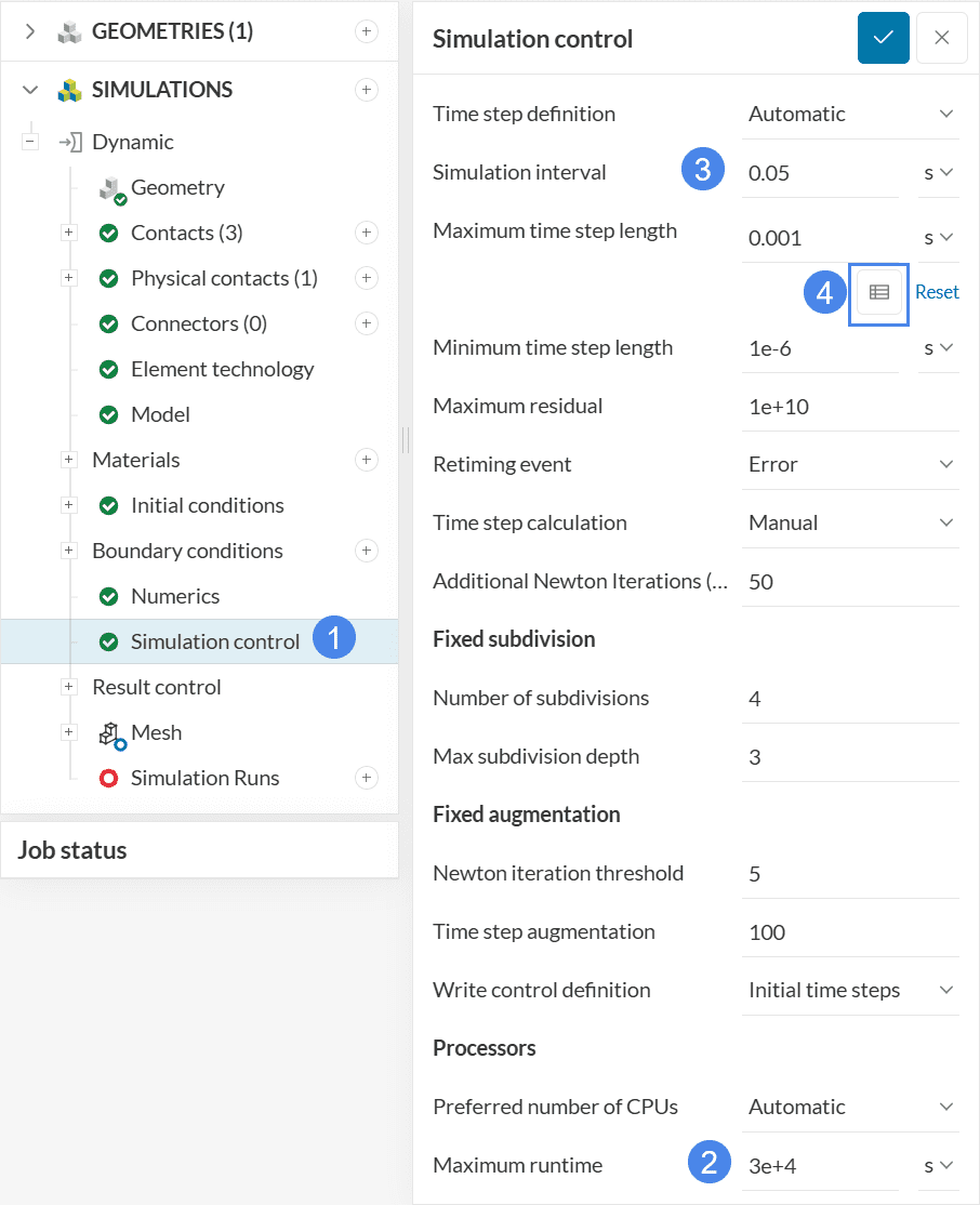
2.5. Simulation Control
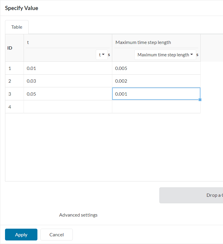
To better capture the impact, some simulation control settings will be changed. Adjust the Simulation interval to ‘0.05’ seconds, and the Maximum runtime to ‘30000’ seconds. To capture the impact more precisely, the Maximum time step length will be defined via a table:
With the settings below, the simulation will have timesteps of:
- 0.005 seconds from t = 0 until t = 0.01 s
- 0.002 seconds from t = 0.01 until t = 0.03 s
- 0.001 seconds from t = 0.03 until t = 0.05 s
2.6. Result Control
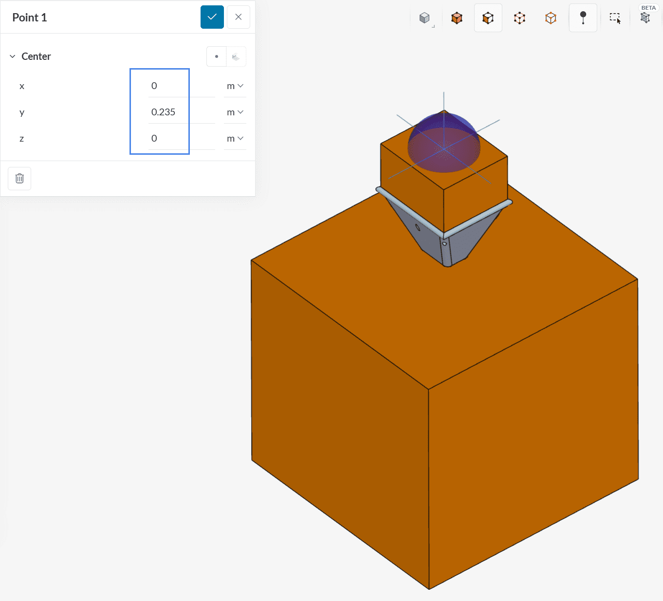
Within Result control, the user can define additional monitors/outputs for the simulation run. Please create a Point data within the Result control tab. The first point will monitor the ‘Acceleration’ on the top of the lead volume:
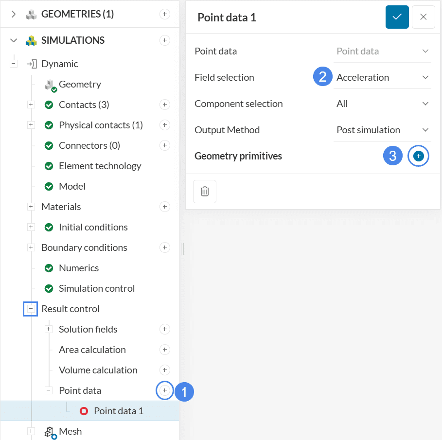
The first point will maintain coordinates 0 for X and Z. The coordinate in Y will be changed to ‘0.235’ meters. When saving the point definition, it will be assigned to the Point data 1 result control.
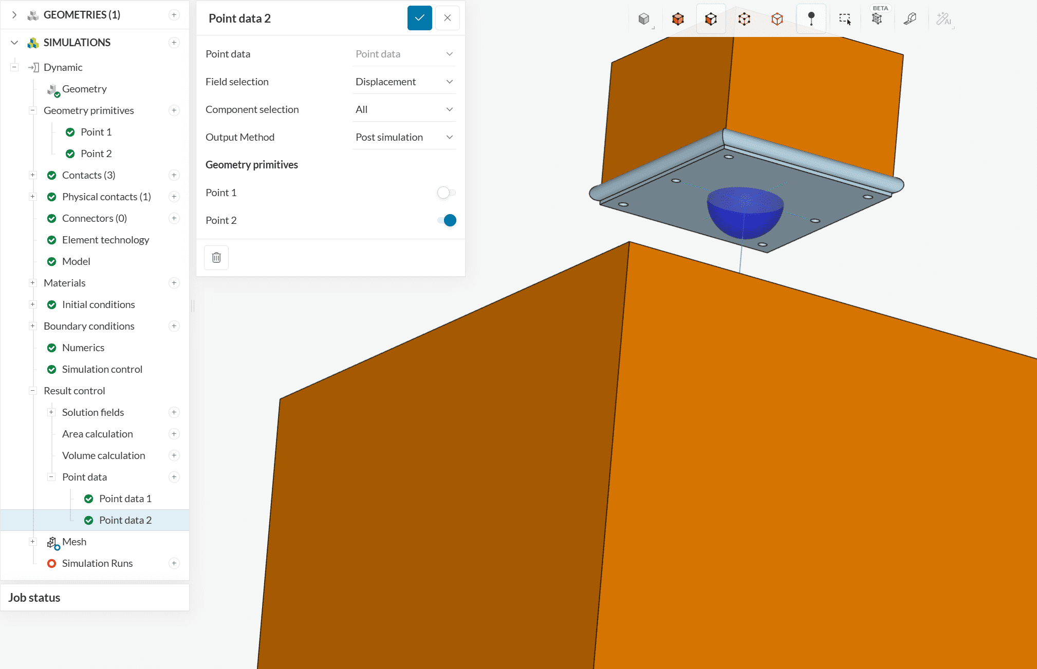
Create a second point data result control, this time selecting ‘Displacement’ for the field. The coordinates for the second point will remain default (0, 0, 0):
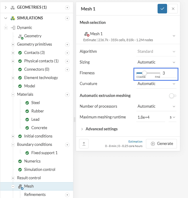
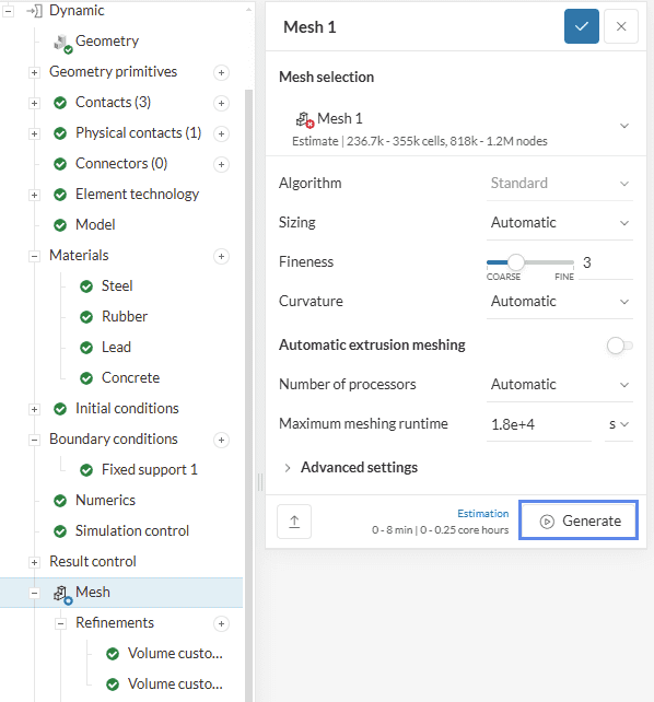
3. Mesh
The standard mesh will be used with an Automatic sizing and Fineness of ‘3’:
Before generating the mesh, some volume refinements will be added to the impact regions, to better capture the collision.
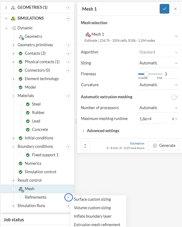
3.1. Volume Custom Sizing
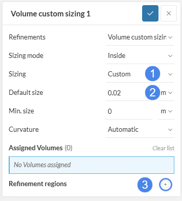
To create a new refinement mesh, click on the ‘+’ button next to Refinements. From the window that comes up, select a ‘Volume custom sizing’:
In the configuration window, you can adjust the Sizing from Automatic to Custom and then modify the Default size of the cells inside the region of interest. For the first refinement, a Default size of ‘0.02’ meters will be applied to a ‘Cartesian box’:
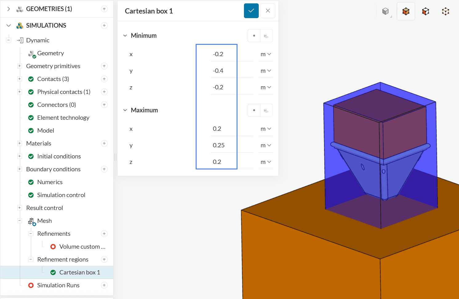
The first volume refinement will be applied to a cartesian box with the following coordinates:
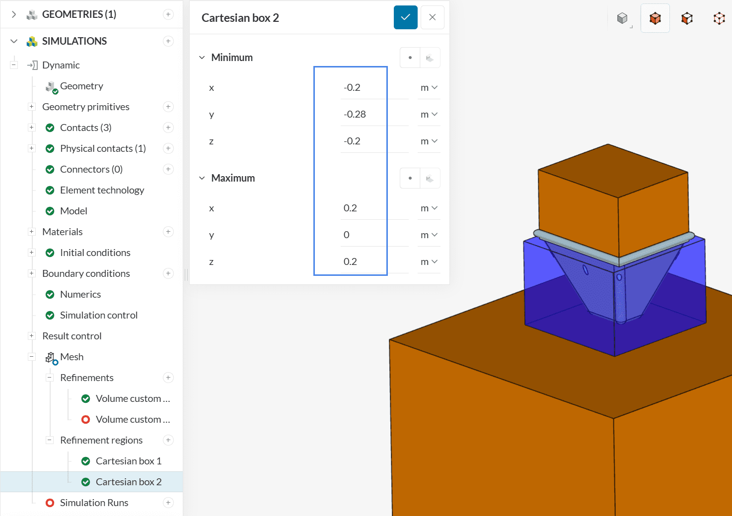
After saving the first coordinates, add another cartesian box, this time for the impact region:
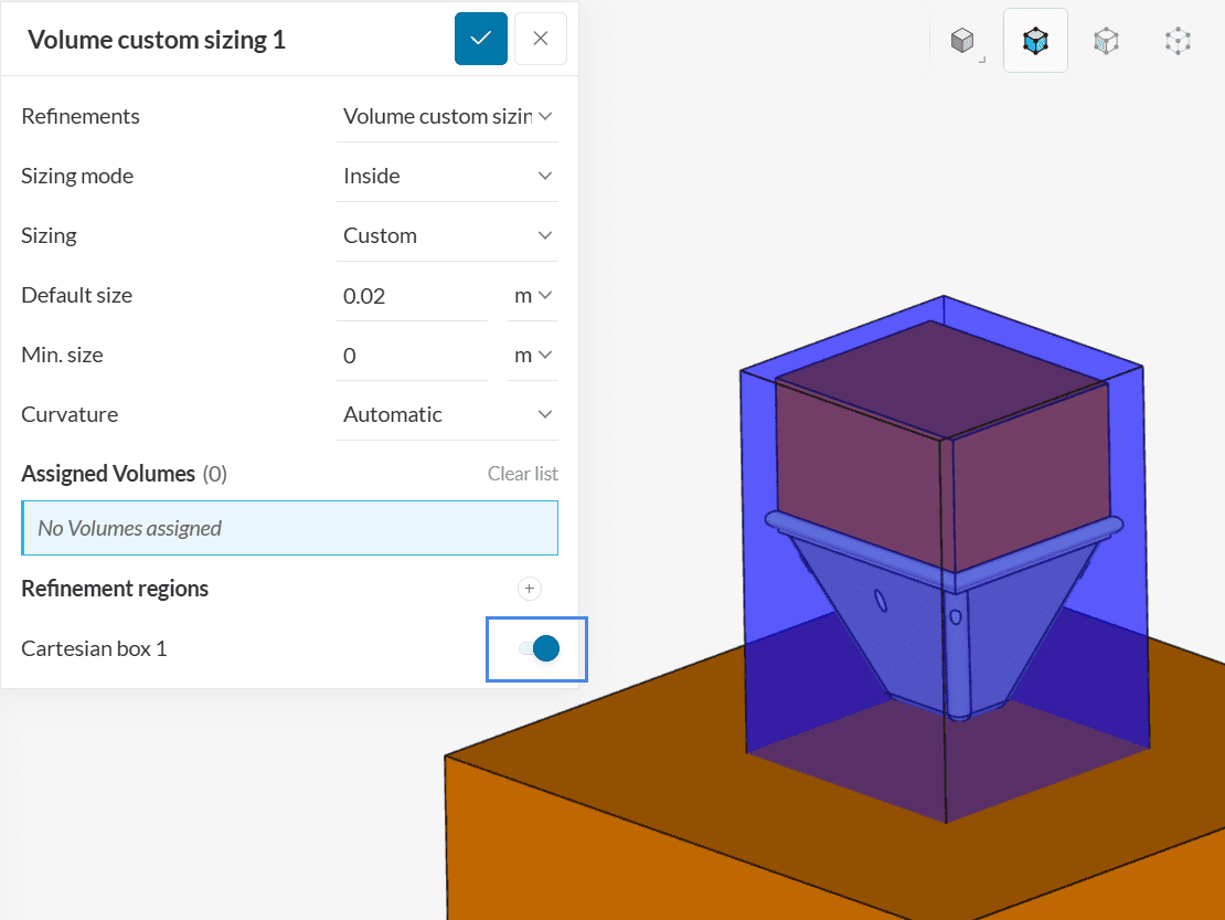
After saving the coordinates of the second box, make sure that both are assigned to the first volume refinement region.
Finally, create another volume custom sizing refinement, this time with a Default size of ‘0.01’ meters, assigned to the cartesian box below:
After assigning the second volume sizing to the impact attenuator cartesian box, open the Mesh tab and ‘Generate’ a new mesh.
4. Start the Simulation
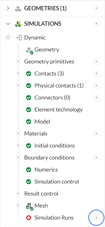
To create a new simulation run, please click on the ‘+’ button next to the Simulation Runs.
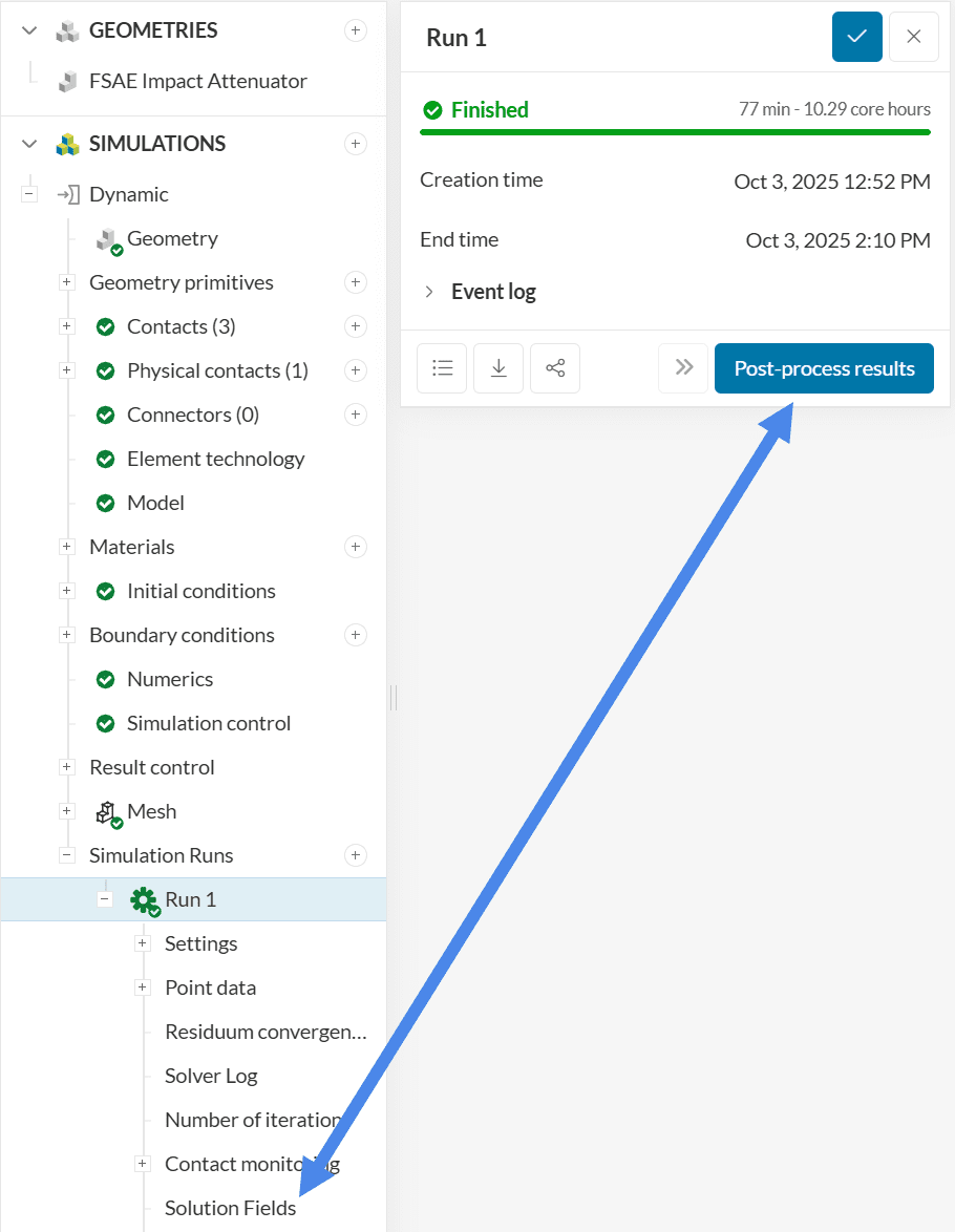
5. Post-Processing
Once the simulation run is finished, you can post-process the impact analysis results. To access the online post-processor you can use one of two methods:
5.1 Visualize the Stress
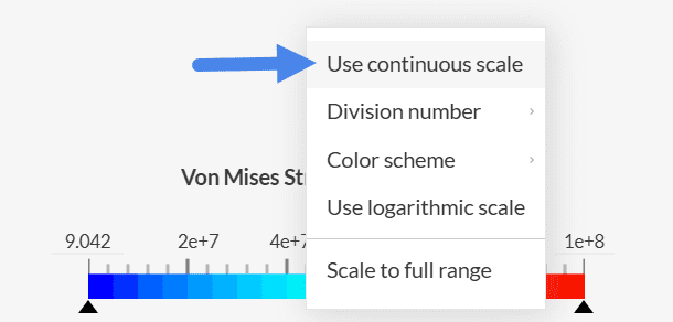
You can notice that the default visualization state shows the Von Mises Stress contour over the geometry. Nonetheless, we can improve the visualization by tweaking the upper legend bound:
Initially, adjust the upper legend bound to ‘1e8’ Pascals. Furthermore, you can also right-click on the legend bar to set a ‘Continuous scale’:
Finally, to better inspect the stress in the interior of the attenuator, we can create a cutting plane. On the top Filters ribbon, click on the ‘Cutting Plane’ icon and adjust its Orientation to ‘X’:
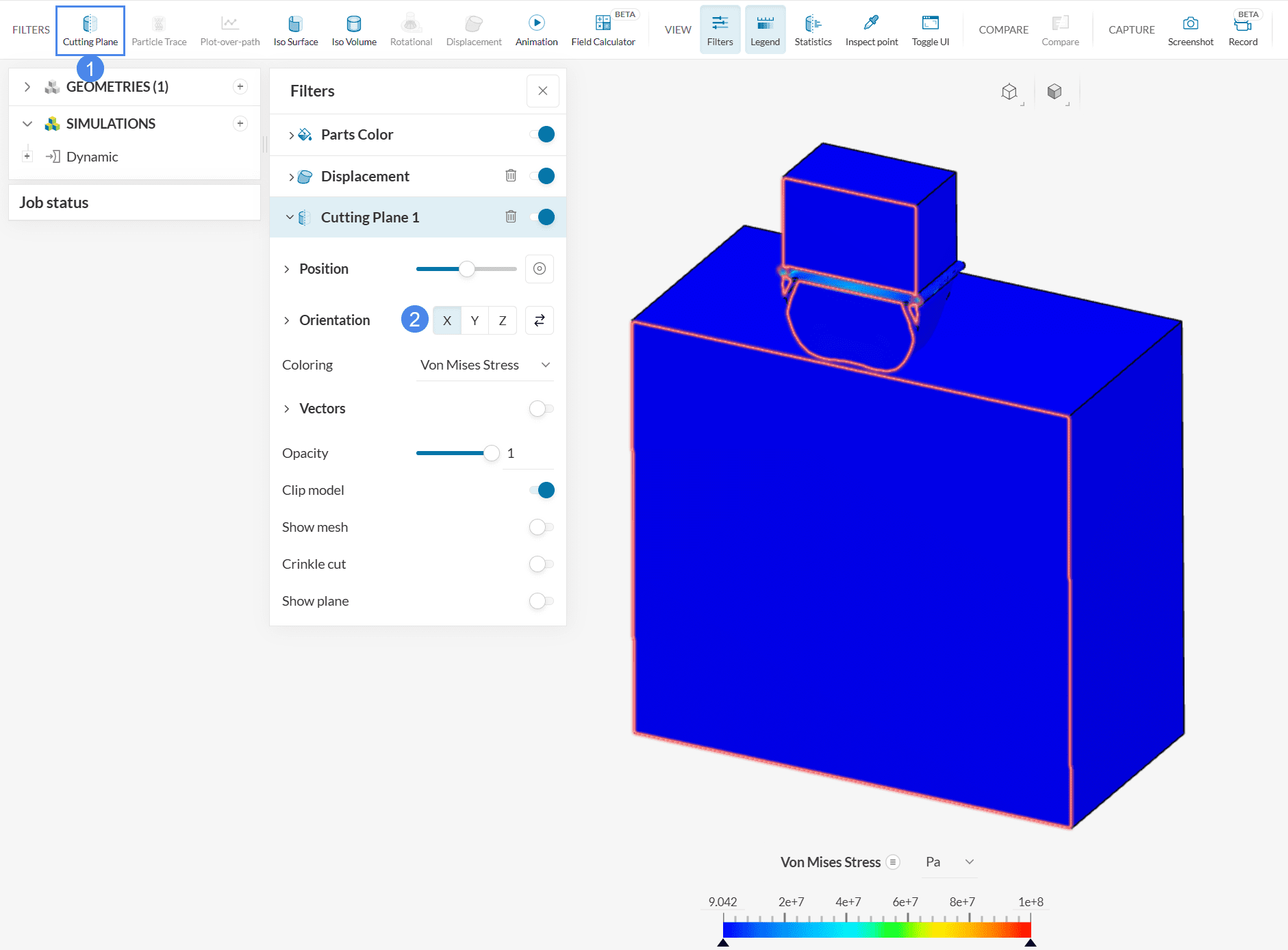
Now you can rotate and zoom the viewer to inspect the stress distribution on any cutting plane of interest.
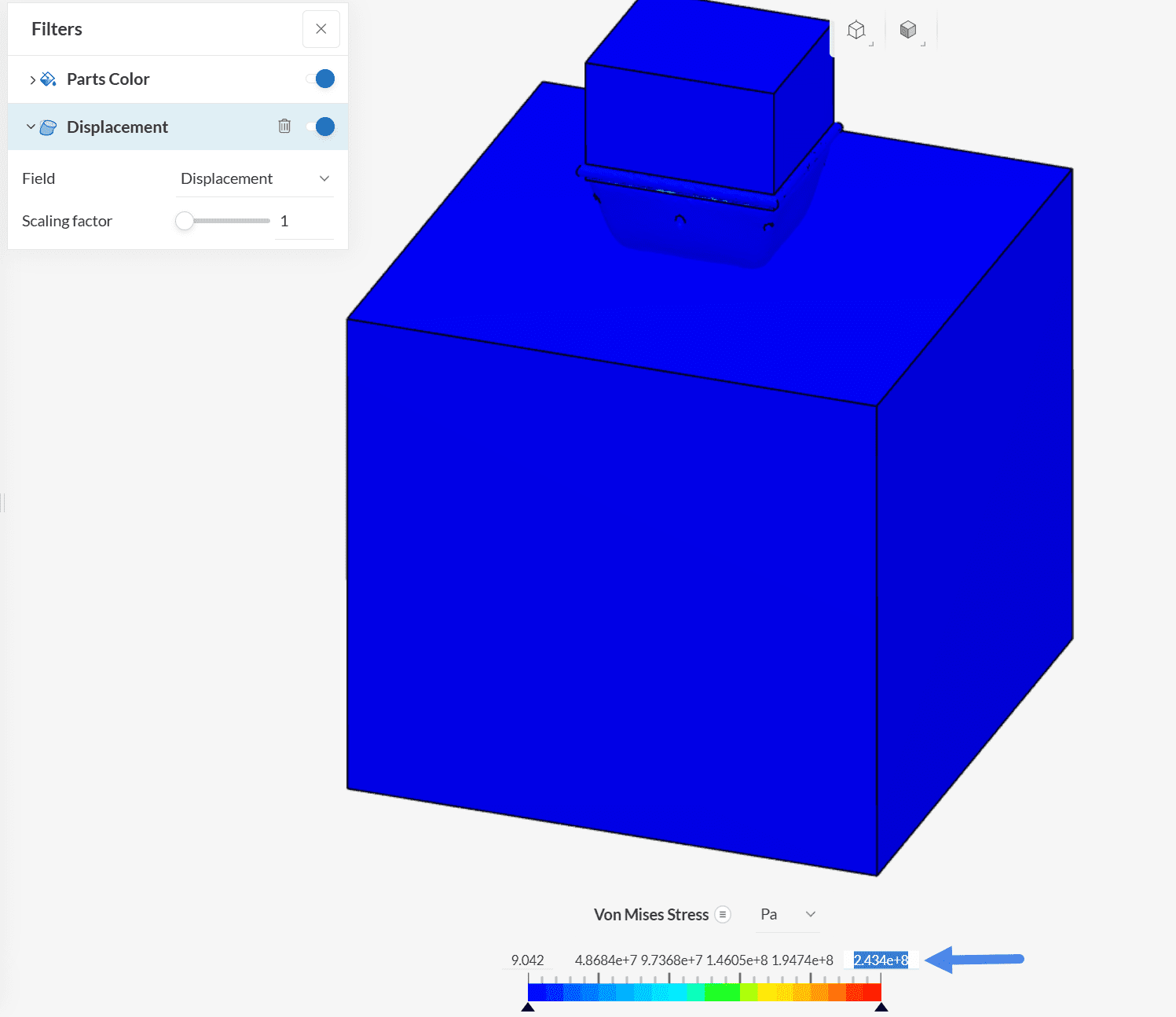
5.2 Displacements
You might have noticed that the default visualization also included a Displacement filter. This filter allows us to see the movement and deformations in the parts. If it is not added already, please go ahead and add the ‘Displacement’ field from the top ribbon.
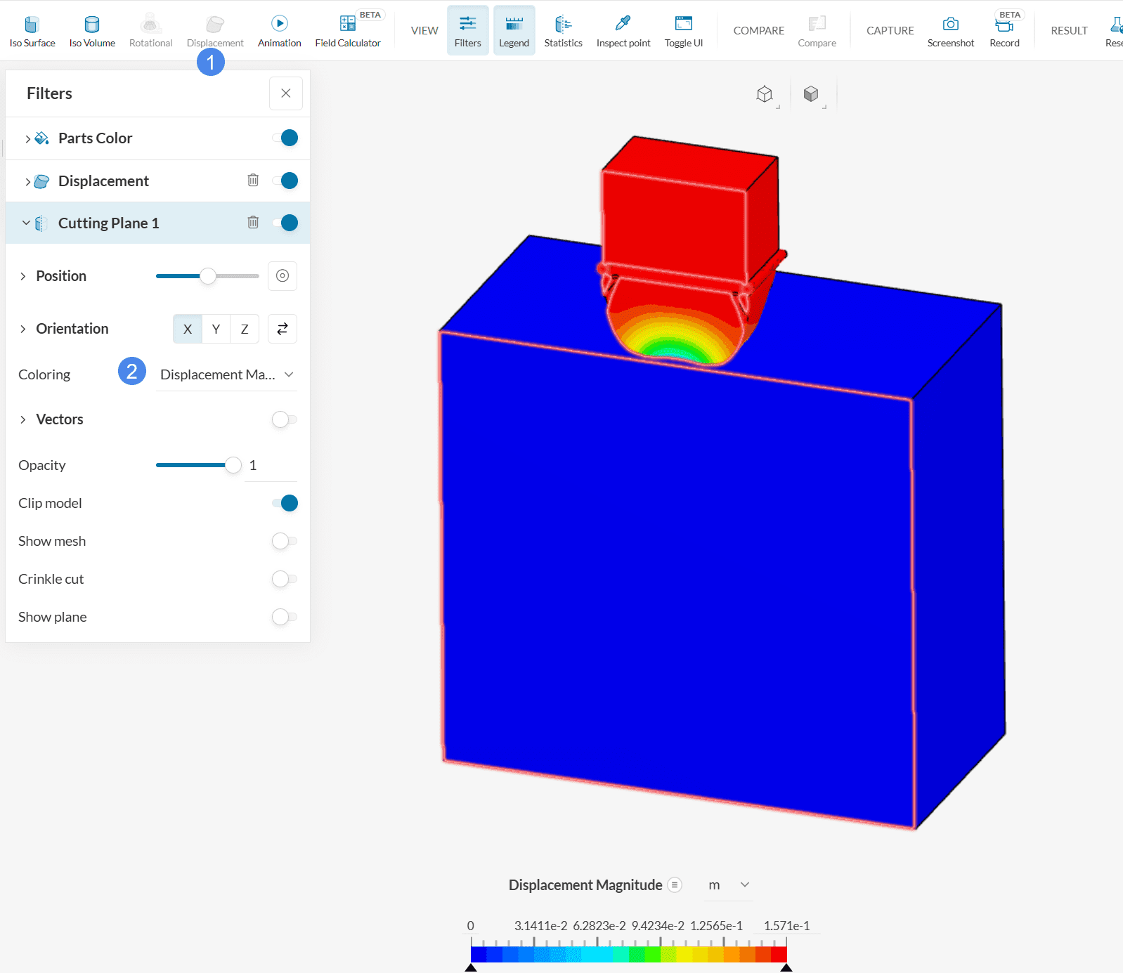
After making sure that the Displacement filter is created, change the Coloring from the Cutting Plane 1 and Parts Color to ‘Displacement magnitude’. By using the Steps bar on the right-hand side panel, you can go through the various timesteps that were saved from the simulation.
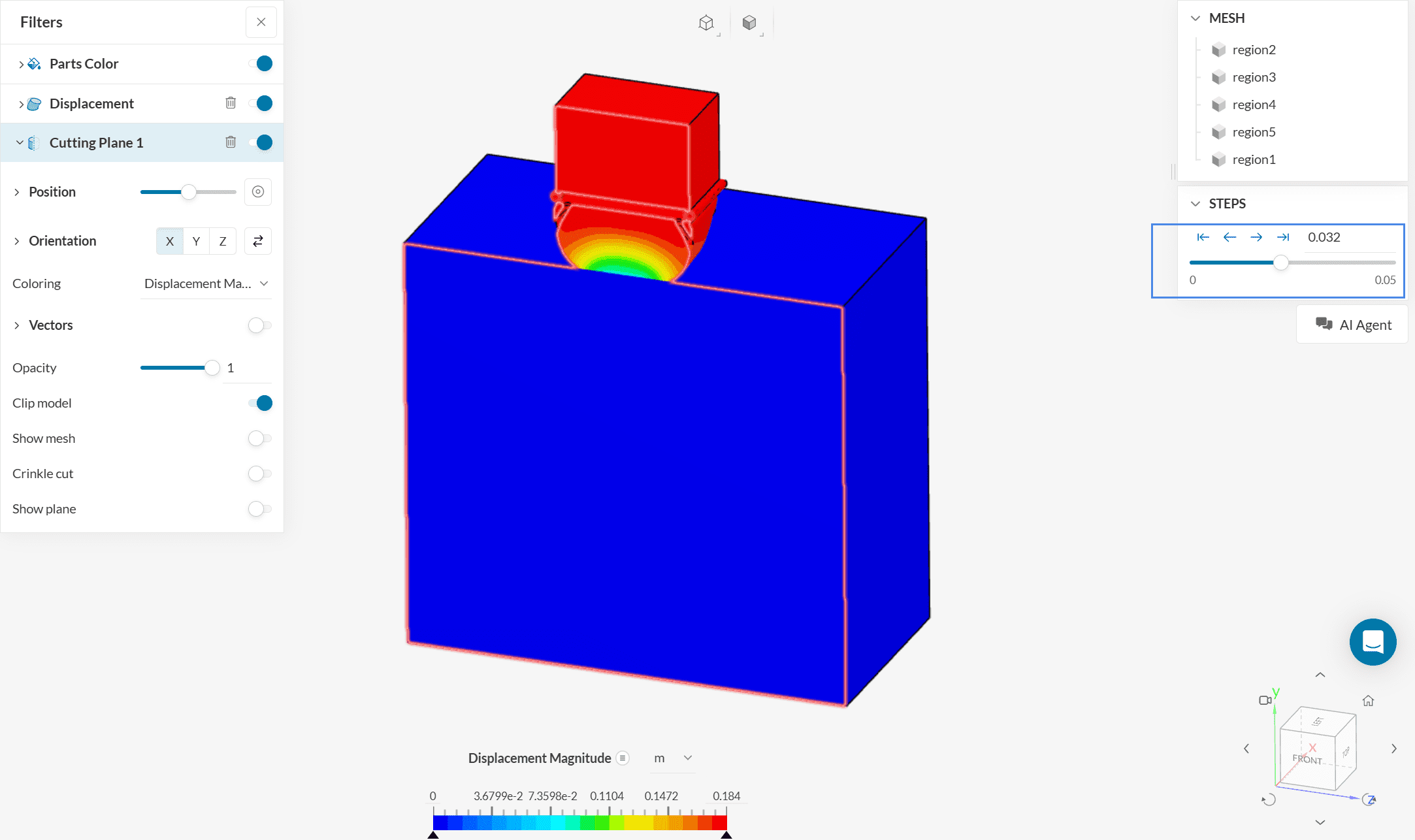
When going through the timesteps, we find that the point of maximum compression is at step 0.036 \(s\), and we can appreciate the displacement distribution, especially on the impact attenuator part.
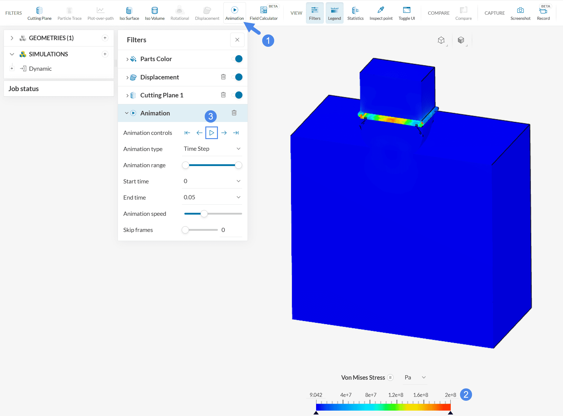
5.3 Impact Test Animation
The whole deformation process can be better visualized by creating an Animation filter. Adjust the Coloring of all components back to ‘Von Mises Stress’ – you may also adjust the upper legend if you want, to improve the visualization of stress gradients. Then, set the animation to play to observe the physics of the collision:
Once an animation is created, it is possible to output a recording by using the Record capture feature:
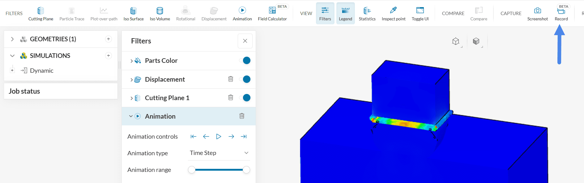
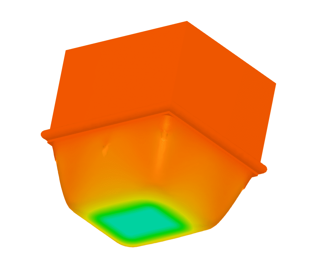
Find below a gif version of the animation, created with the Record feature.
The deformations and stress evolution of the parts can be appreciated in context thanks to the animation. Regions colored in yellow and red show the development of higher stress values.
Analyze your results with the SimScale post-processor. Have a look at our post-processing guide to learn how to use the post-processor.
Congratulations! You finished the tutorial!
Note
If you have questions or suggestions, please reach out either via the forum or contact us directly.
Last updated: October 20th, 2025
Did this article solve your issue?
How can we do better?
We appreciate and value your feedback.


