\underline{\textbf{Introduction}}
Turbulent boundary conditions are often overlooked in simulation and left as default, which can lead to inaccurate results in many cases. Turbulent boundary conditions can be calculated using experimental results, but in most cases, it is enough to approximate them based on our understanding of flows and information about the domain to be simulated.
\underline{\textbf{Impact of Turbulent Boundary Conditions on Results}}
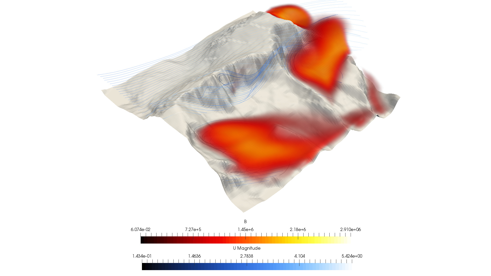
Figure 1: Simulation of flow around a mountain, volume rendering showing \beta, and streamlines showing speed and direction of flow. CAD model kindly provided by Rrett Thys from GrabCAD.
The above simulation illustrates turbulence generated by a flow around a mountain, showing that if you wanted to place a domain at a location on this mountain—for wind generation, for example—the turbulent boundary conditions may vary dramatically upon domain placement. On the flow side of the mountain, there is little turbulence and therefore the inlet conditions can reflect that. If placed on the wake side, however, the turbulence of the flow needs to be better approximated. Furthermore, if the wind was blowing in a different direction, the clean flow that was present in another condition might become very turbulent and completely change the results.
Depending on your case, the effects of turbulence in the freestream may alter your results in different ways and with different magnitudes. Take this aircraft, flying at about 97 knots with different turbulent inlet conditions. We can see that the amount of total drag is largely influenced by skin friction, accounting for approximately a quarter:
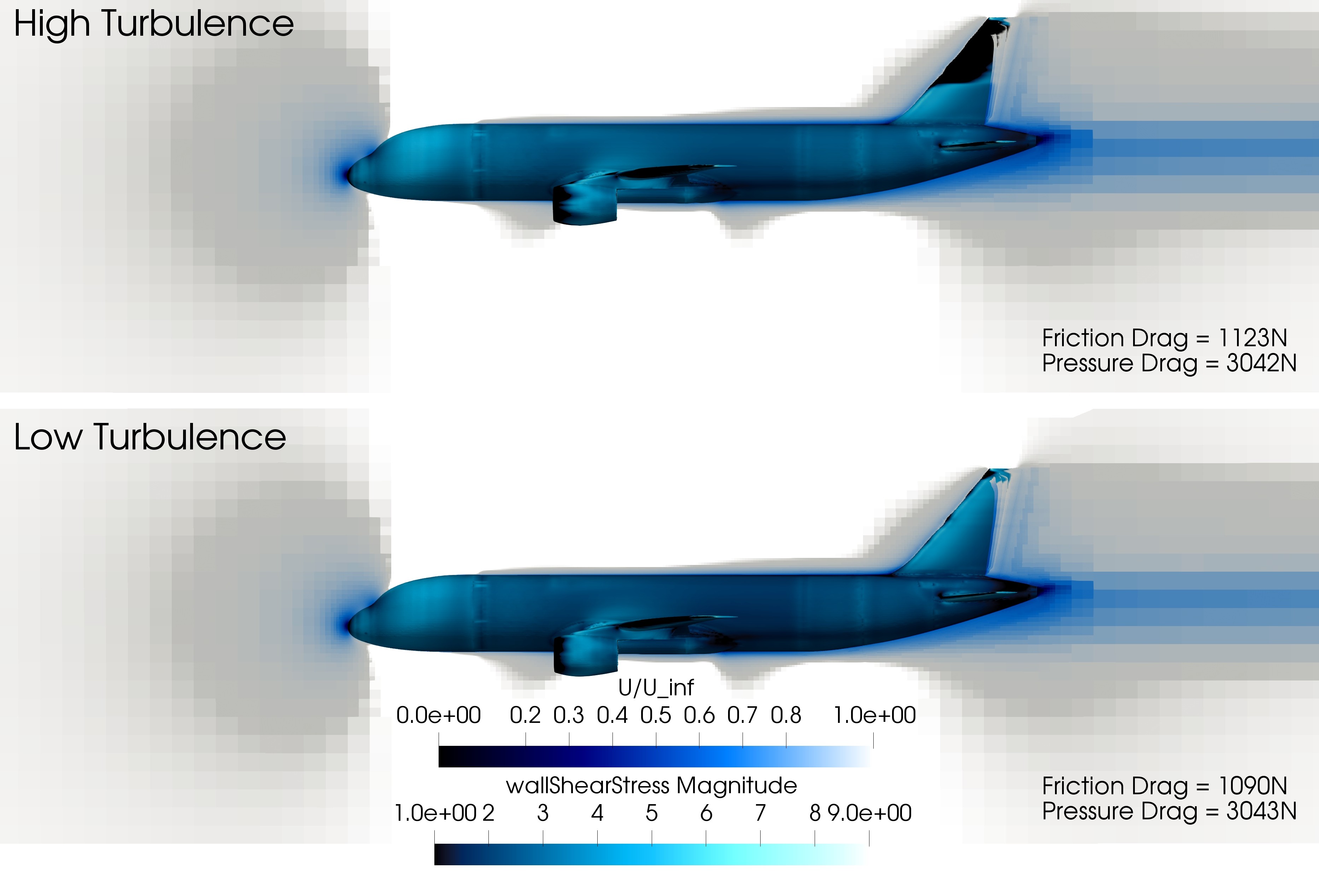
Figure 2: The same aircraft traveling through a highly turbulent freestream (top) and through a low turbulent freestream (bottom). The planar slice shows U/U_\infty and the surface of the aircraft displays wall shear stress.
The pressure drag barely decreases in this simulation because there is very little separation. The friction drag, however, has increased by about 33N making the total increase in drag about 32N or in perspective a 0.5% increase in total drag at higher turbulence. But looking at these images, it is very hard to figure out where this increase comes from. At the top surface of the aircraft, the boundary layer can be clearly seen in faint blue. Comparing the difference between low and high turbulence results, it can be seen that in the high turbulence simulation the boundary layer is actually thicker (visible by the intensity of blue). This is because turbulent boundary layers are much thicker and the earlier transition to a turbulent layer gives the layer more length to expand over.
Taking a different case, one that is dominated by pressure drag:
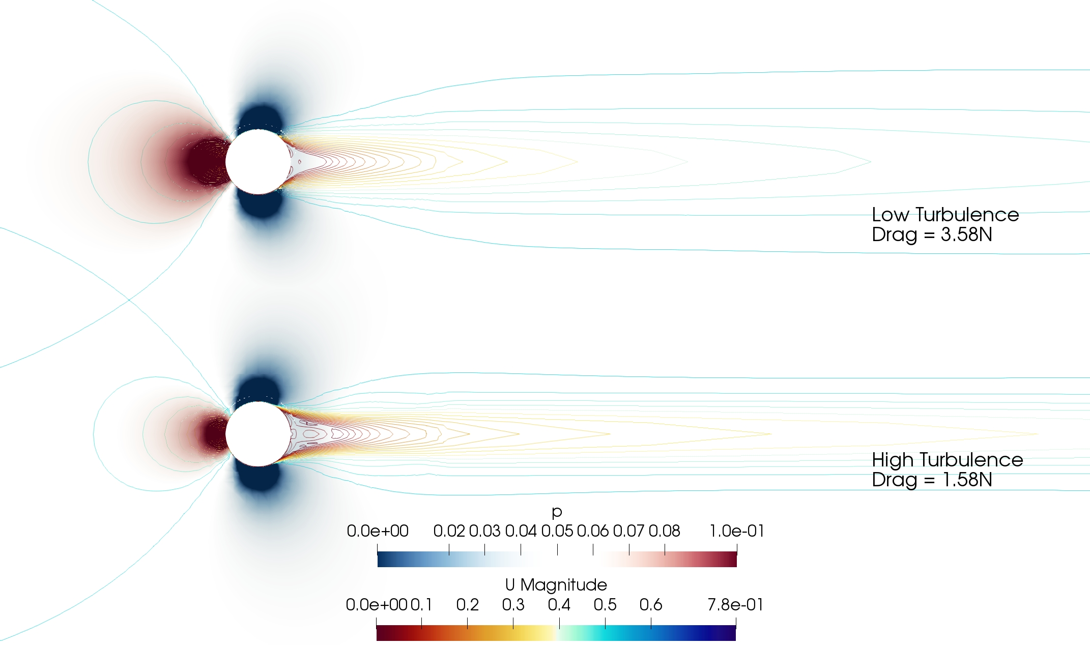
Figure 3: Reduction in wake width, reducing the pressure difference
Immediately visible is the pressure difference at the leading edge between the low and high turbulence results. This is because the wake behind the cylinder has been reduced in width and therefore puts up less resistance to flow around it. This is very visible from the post-processing images above. The wake has been caused by flow separation, and this flow separation happens when there is an adverse pressure gradient in the boundary layer. What makes the difference, however, is the level of turbulence—the higher the turbulence, the better the boundary layers’ ability to remain attached to the surface and therefore separation is held off. Consequently, if flow entering the domain is of higher turbulence, it is likely that the flow around the cylinder will also be higher.
A final factor to consider when defining turbulence at the boundary is that turbulent energy dissipates over time; this will be true for turbulence in the inlet. Thus the bigger the distance between the inlet and the object being simulated, the less turbulent the flow at the object. This might mean that increasing the turbulence at the inlet has no effect at all on the results, which might be desirable depending on your application.
\underline{\textbf{ Turbulent Boundary Conditions in SimScale}}
This quote is taken from the SimScale documentation about velocity inlets:
The relevant turbulent flow quantity values are taken the same as the initial field values.
To define the correct turbulent boundary conditions, you must treat the initial conditions as the inlet conditions also. It is perfectly acceptable to have the turbulent initial conditions identical to the inlet conditions. However, it is recommended on some online resources that they are set 10 times the inlet values. This is because turbulence within the system is expected to be much greater than at the inlet. Setting this to high will allow the system to settle instead of constantly increasing the conditions until they are correct. Although 10 times is recommended, you can make your own decision. To use this method of setting the initial conditions higher than the inlet conditions, the user will be required to create a custom boundary condition where the velocity is an inlet—the turbulent values at the boundary are fixed, however.
\underline{\textbf{External Flow Approximations }}
External flows can be a bit tricky to approximate because it is hard to evaluate the flow downstream taking into account anything that could have affected the turbulence. This could be other objects, convection over land or the position of the domain in a boundary layer. A good technique for approximation turbulence is by using the Turbulent Viscosity Ratio—the ratio between molecular viscosity and turbulent viscosity. This ratio can be used along with the Turbulence Intensity, freestream velocity and molecular viscosity to determine k, \varepsilon and \omega using the following technique.
To start the calculation, the Turbulent Intensity I, and Viscosity Ratio \boldsymbol{\beta} need to be approximated by using the table below.
To calculate k, the following equation can be used:
Calculating k is a good starting point as it can be used along with the Eddy Viscosity Ratio \boldsymbol{\beta}, Molecular Viscosity and density to calculate both \boldsymbol{\varepsilon} and \boldsymbol{\omega} using equations:
\underline{\textbf{ Approximation Table}}
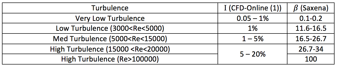
Figures are taken from two sources, I have interpreted the scale of turbulence (low, medium, etc.) for the Reynolds number.
\underline{\textbf{Internal Flow Approximations}}
\textbf{Fully-developed Flow}
For a fully-developed inlet flow, approximating turbulent boundary conditions can be carried out with some certainty.
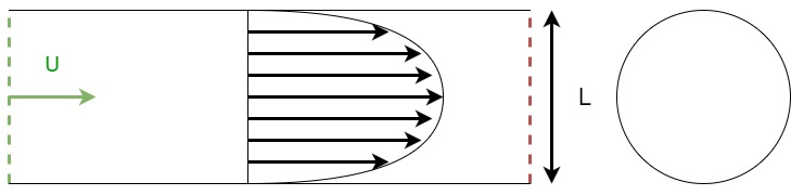
Using the Reynolds number to determine the intensity and the diameter as the characteristic length \textbf{L} to define the intensity length scale \textbf{l}, the required turbulent boundary conditions can be calculated.
Where \textbf{U} is average velocity in the pipe or duct, \textbf{L} is the diameter of the pipe or hydraulic diameter of the duct, and \boldsymbol{\nu} is the kinematic viscosity of the fluid. This can be used to determine the turbulent intensity.
This can be used to calculate a mean approximation for the turbulent boundary conditions k, \omega and \varepsilon using the equations:
Where the turbulent length scale l is defined using the approximation:
Internal flows are rarely that simple, but by breaking the inlets down into components and approximating each inlet individually, the simulation will do the rest. Take this turbulent jet with a cross flow problem:
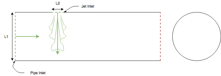
By using the same equations, we can approximate the Reynolds number for the jet, and a Reynolds number for the pipe inlet. This is a good example of how using the initial conditions as the turbulent boundary condition values might be a bad approximation, because the turbulence from each flow will be very different.
\underline{\textbf{Modified Turbulent Viscosity, NuTilda,}\quad \widetilde{\nu}}
A Spalart and Allmaras Large Eddy Simulation term, \widetilde{\nu} is required, for laminar flow setting this to zero is ideal, if numerical dificaluties arrise then it can be set low as \widetilde{\nu} \leq \frac{\nu}{2} without effecting the laminar regions (P. R. Spalart, and S. R. Allmaras, 1994). Else if fully turbulent then \widetilde{\nu} can be treated as 2\nu < \widetilde{\nu} < 3\nu (NASA, 2016), where full turbulence will be pressumed in regions of shear.
\underline{\textbf{Turbulent/Eddy Kinematic Viscosity, Nut, }\quad \nu_t}
In the Spalart and Allmaras Large Eddy Simulation model {\nu}_t should correspond to \widetilde{\nu} as {\nu}_t = 0 and 0.210438\nu < \nu_t < 1.294234\nu (NASA, 2016).
\underline{\textbf{Online Calculators}}
There are many online calculators which will turn known parameters into turbulent boundary condition values. The most comprehensive and diverse is the tool provided on CFD Online. Not only is it handy, but it also provides a lot of information about the parameters and is highly recommended for further reading. Please see the link below:
CFD Online - Turbulence Properties, Conversions & Boundary Estimations
\underline{\textbf{Symbols}}
\boldsymbol{k} = Turbulent kinetic energy
\boldsymbol{\omega} = Specific turbulent dissipation rate
\boldsymbol{\varepsilon} = Turbulence dissipation
\boldsymbol{I} = Turbulent intensity
\boldsymbol{U} = Freestream velocity
\boldsymbol{U_{RMS}} = Root mean square of velocity fluctuations
\boldsymbol{u_x},\boldsymbol{u_y} and \boldsymbol{u_z} = Velocity fluctuations in the x, y and z components
\boldsymbol{\mu}, \boldsymbol{\mu_\tau} = Laminar and turbulent viscosity
\boldsymbol{\beta} = \boldsymbol{\frac{\mu_\tau}{\mu}} = Viscosity ratio
\boldsymbol{\rho} = Fluid density
\boldsymbol{Re} = Reynolds number
\boldsymbol{l} = Turbulent length scale
\boldsymbol{L} = Characteristic length
\boldsymbol{C_\mu} = Model constant (usually 0.09 for k-epsilon)
\underline{\textbf{References and Background Reading}}
Apsley, D. (2017, Spring). Turbulence Modelling. Retrieved from Manchester University: http://personalpages.manchester.ac.uk/staff/david.d.apsley/lectures/comphydr/turbmodel.pdf
CFD-Online (1). (n.d.). Turbulence Intensity. Retrieved from CFD-Online: Turbulence intensity -- CFD-Wiki, the free CFD reference
CFD-Online (2). (n.d.). Turbulence Free-stream Boundary Conditions. Retrieved from CFD-Online: Turbulence free-stream boundary conditions -- CFD-Wiki, the free CFD reference
CFD-Online (3). (n.d.). Reynolds Number. Retrieved from CFD-Online: Reynolds number -- CFD-Wiki, the free CFD reference
CFD-Online (4). (n.d.). Specific Turbulence Dissipation Rate. Retrieved from CFD-Online: Specific turbulence dissipation rate -- CFD-Wiki, the free CFD reference
MIT. (n.d.). Basics of Turbulent Flow. Retrieved from MIT: http://www.mit.edu/course/1/1.061/www/dream/SEVEN/SEVENTHEORY.PDF
Saxena, A. (n.d.). Guidelines for Specification of Turbulence at Inflow Boundaries. Retrieved from esi-cfd: http://support.esi-cfd.com/esi-users/turb_parameters/
P. R. Spalart, and S. R. Allmaras (1994) A One-equation Turbulence Model for Aerodynamic Flows.
NASA (2016) The Spalart-Allmaras Turbulence Model. Available at: Spalart-Allmaras Model
Credits to PowerUser Darren (@1318980).
Contributions and suggestions for improving this page are welcome, please private message @1318980.